The Oregon Zoo in Portland
We drove a couple of hours to visit The Oregon Zoo. I don’t like zoos much, lately, because they house imprisoned animals, but I am aware that they do a lot of good work towards saving endangered animals from extinction. So I was ambivalent about this trip; nevertheless, I was pleasantly surprised at the quality of this particular zoo.
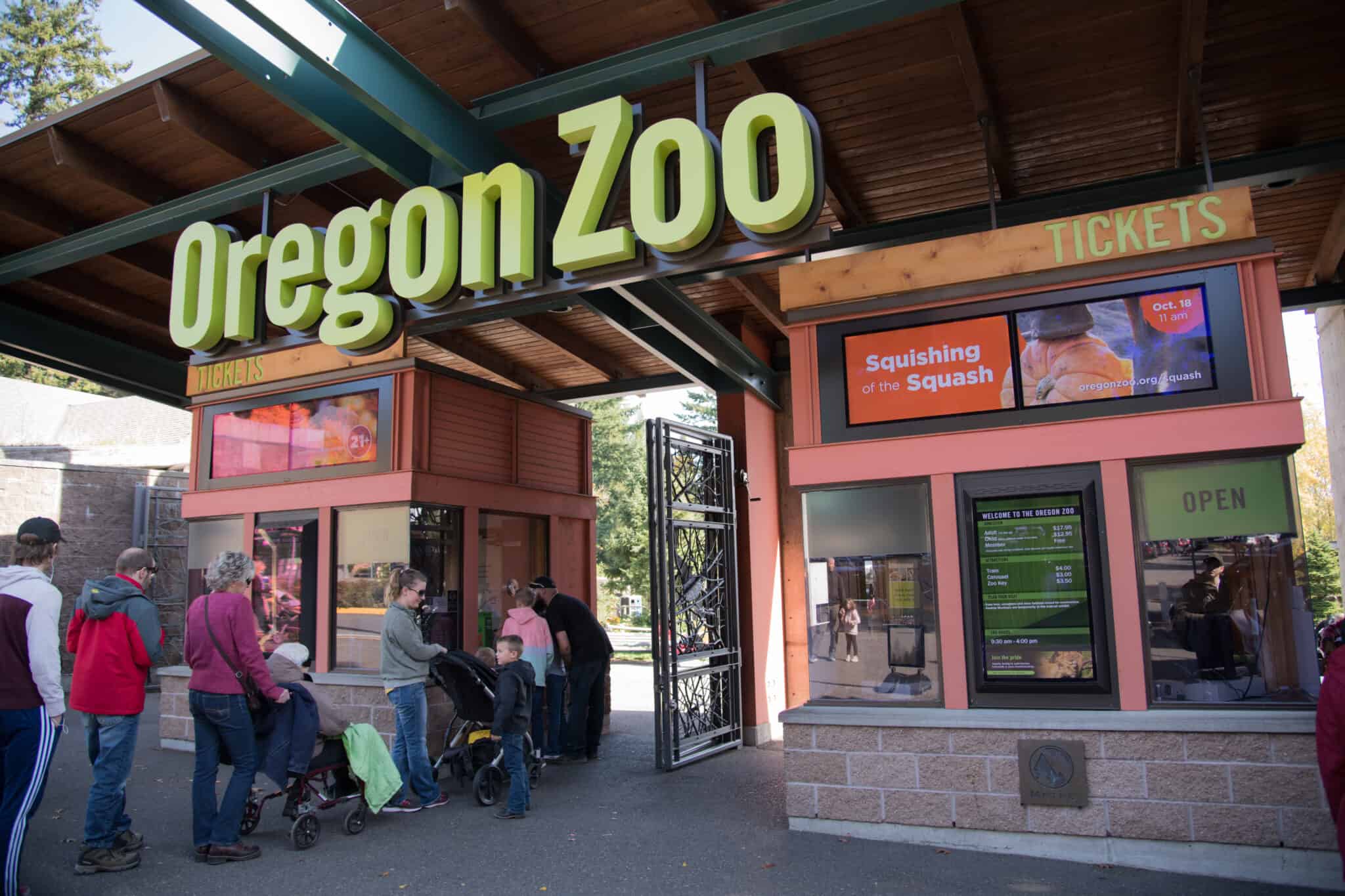
I bought a ticket for the 11:00 a.m. window from a kiosk, which printed my bar code–all without a hitch and no line.
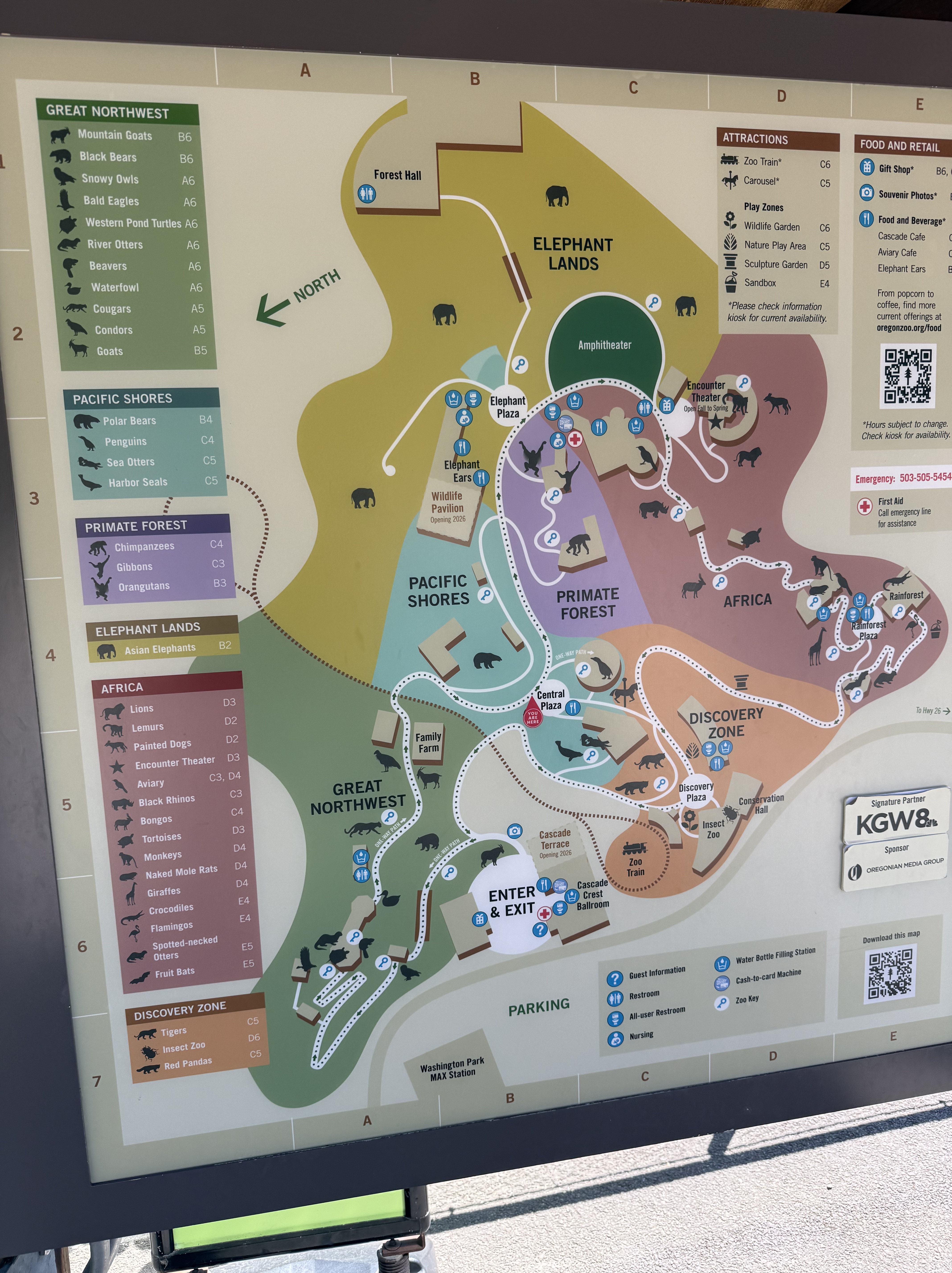
It was a beautiful day, so the parking lot was full; but we parked at the overflow parking lot and rode a free school bus for a quick trip to the entrance. It was better than parking in the regular lots. The arrows show the one-directional flow of people that is encouraged by the layout. It’s about two miles and takes 2-3 hours.
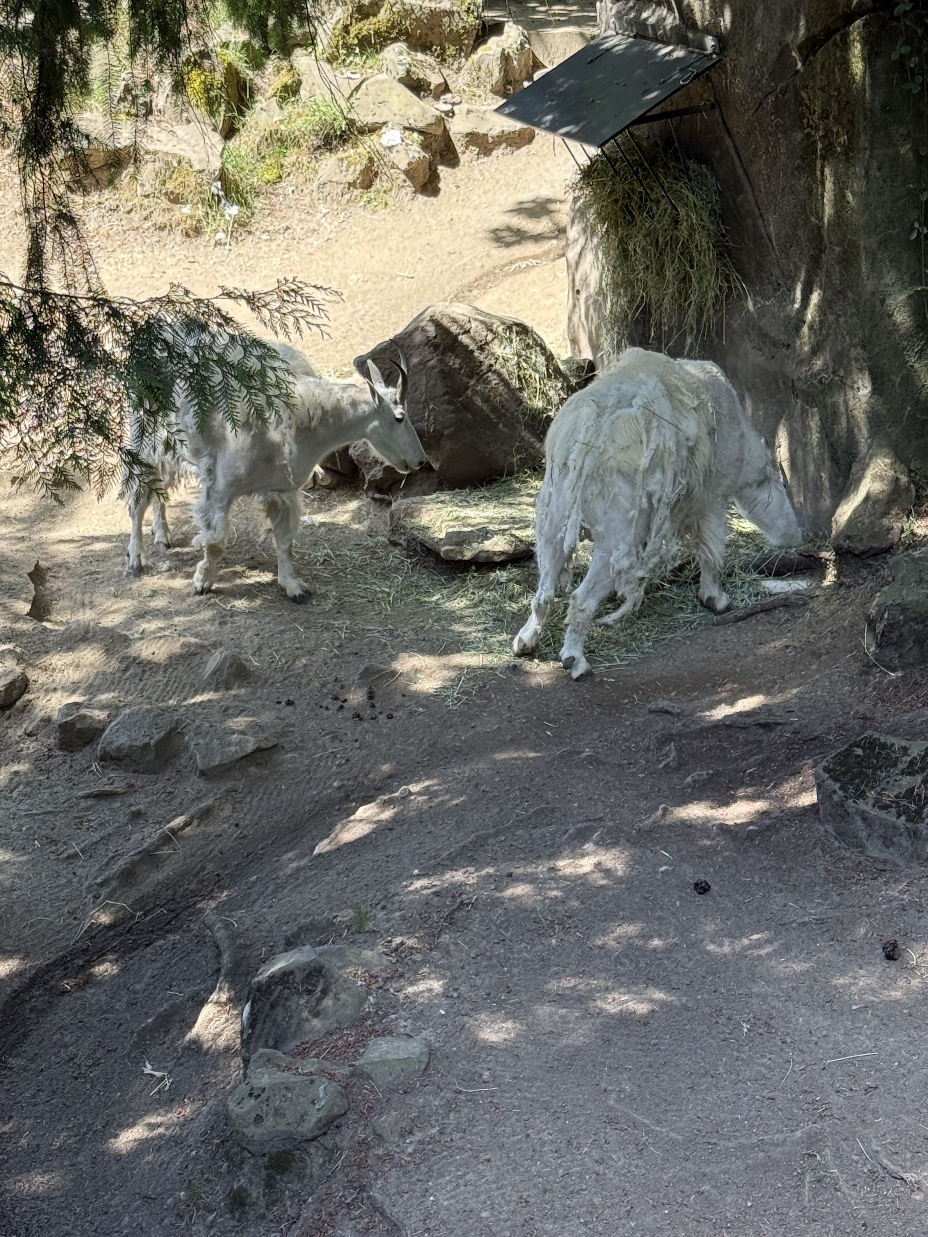
There is a mountain goat exhibit at the entrance with artificial rock piles, but its inhabitants were having lunch. They look pretty ragged, I guess because they’re losing their winter hair (or is it fur?).
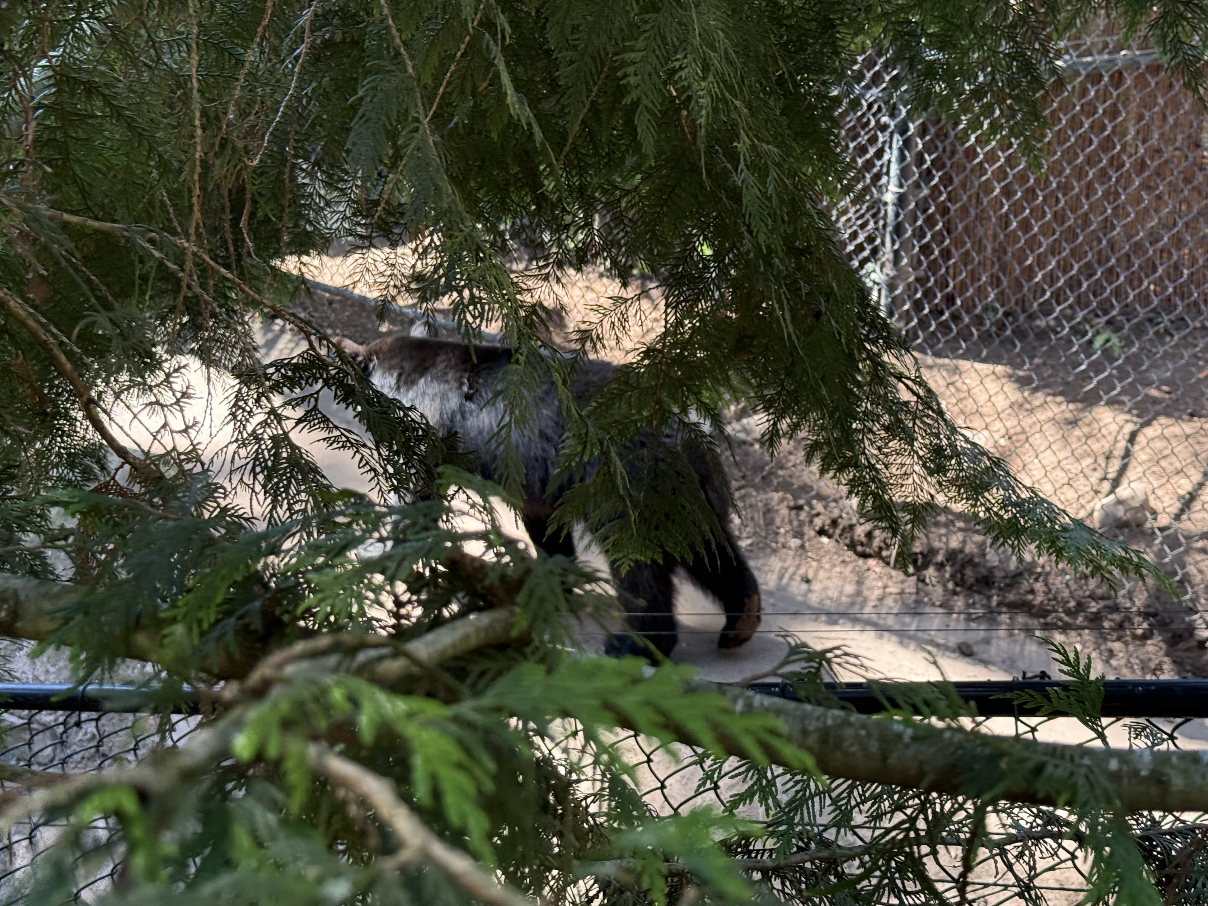
The Pacific Northwest was a grouping of regional species, including three black bears. I missed a lot of opportunities to photograph them interacting because I was confused by their enclosure, which was very large. It covers the side of a hill and includes several personal areas in addition to available shared “dens” where they could get some privacy from prying eyes.
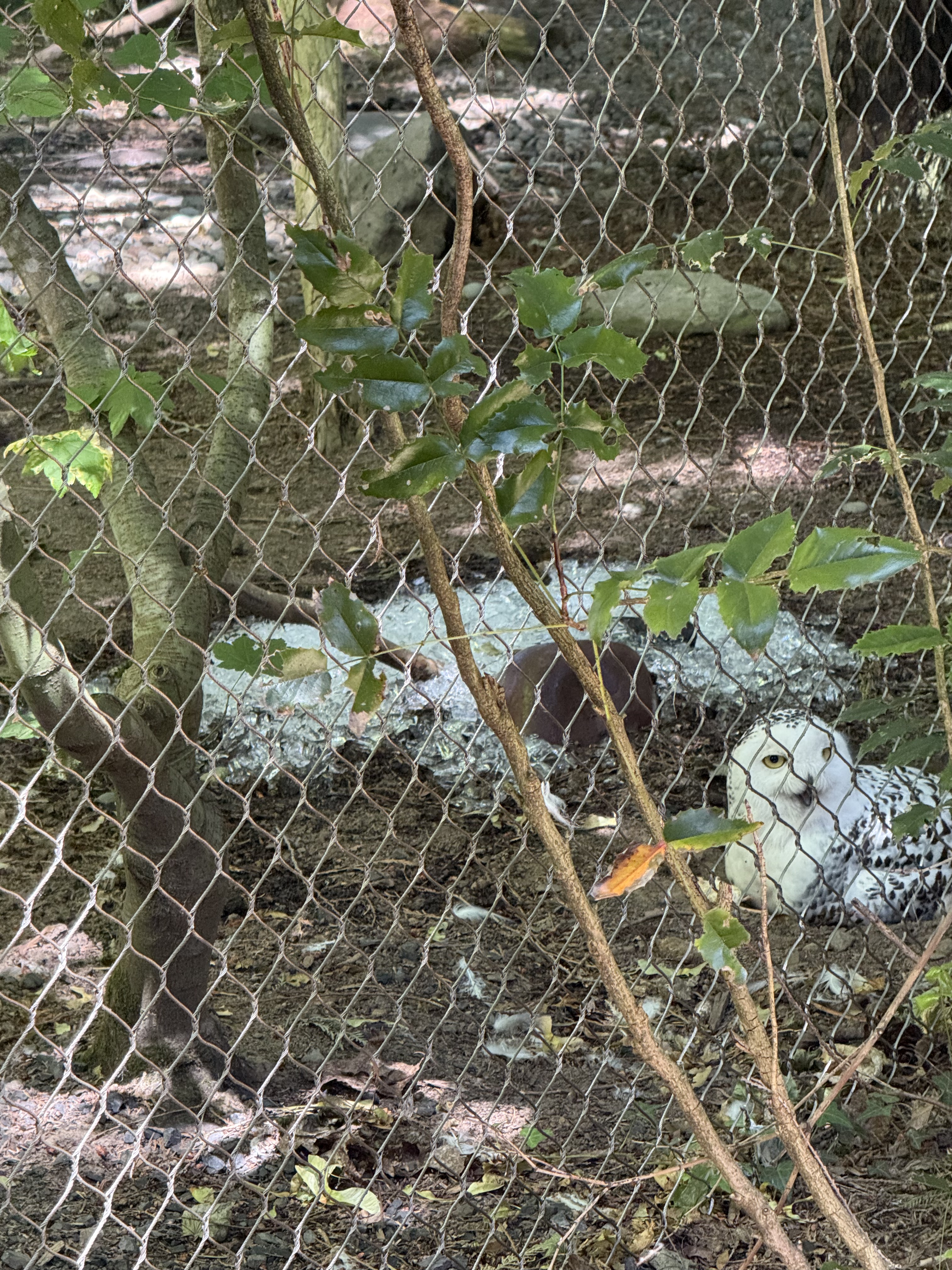
The owls seemed to enjoy sitting on the ground, even on a pile of ice, even though they had plenty of branches to hang out on.
There was plenty of shade available for the inhabitants as well as the visitors.
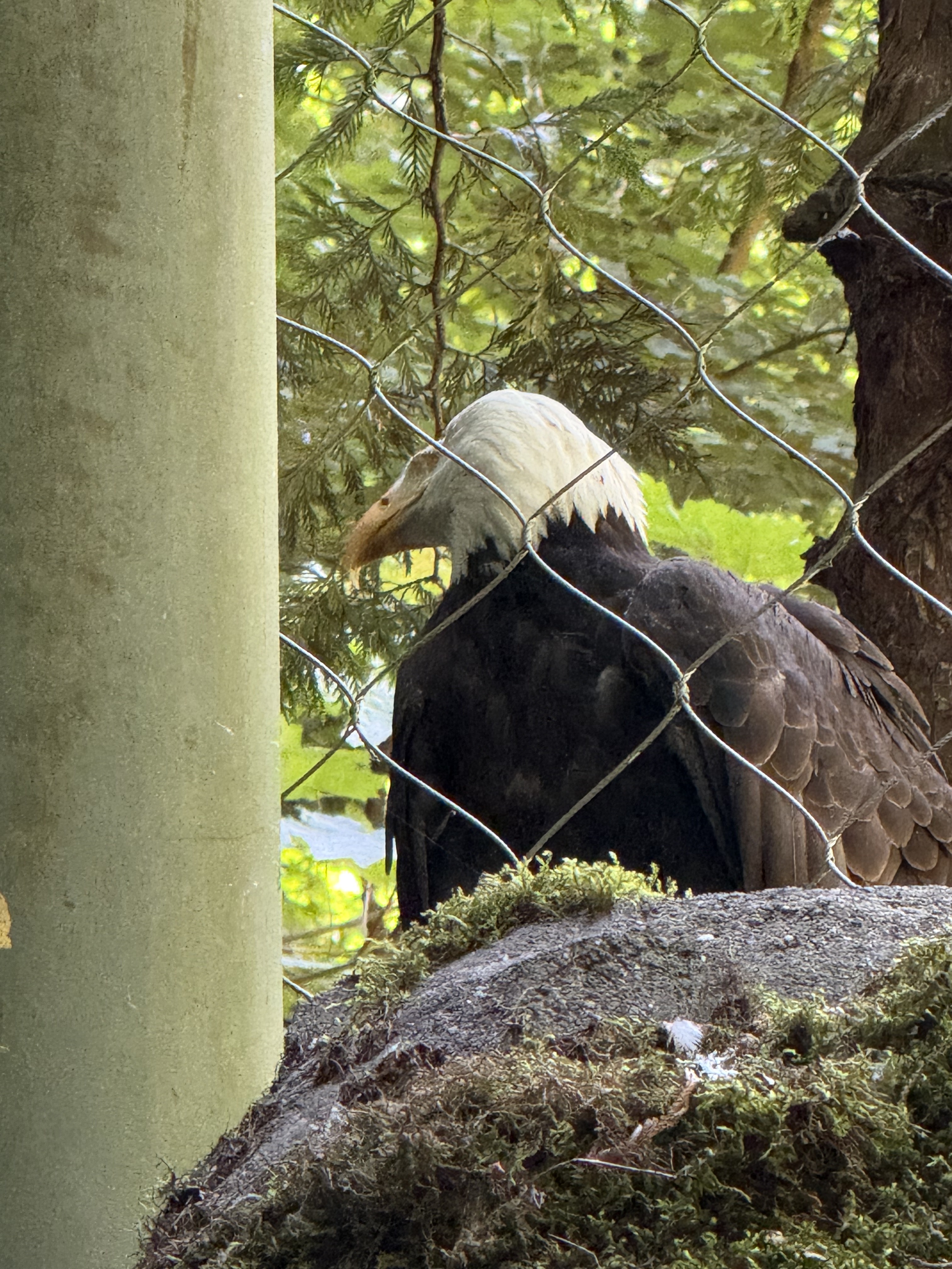
The bald eagles were rescued and are unable to fly properly, so I guess this is an “assisted living” facility.
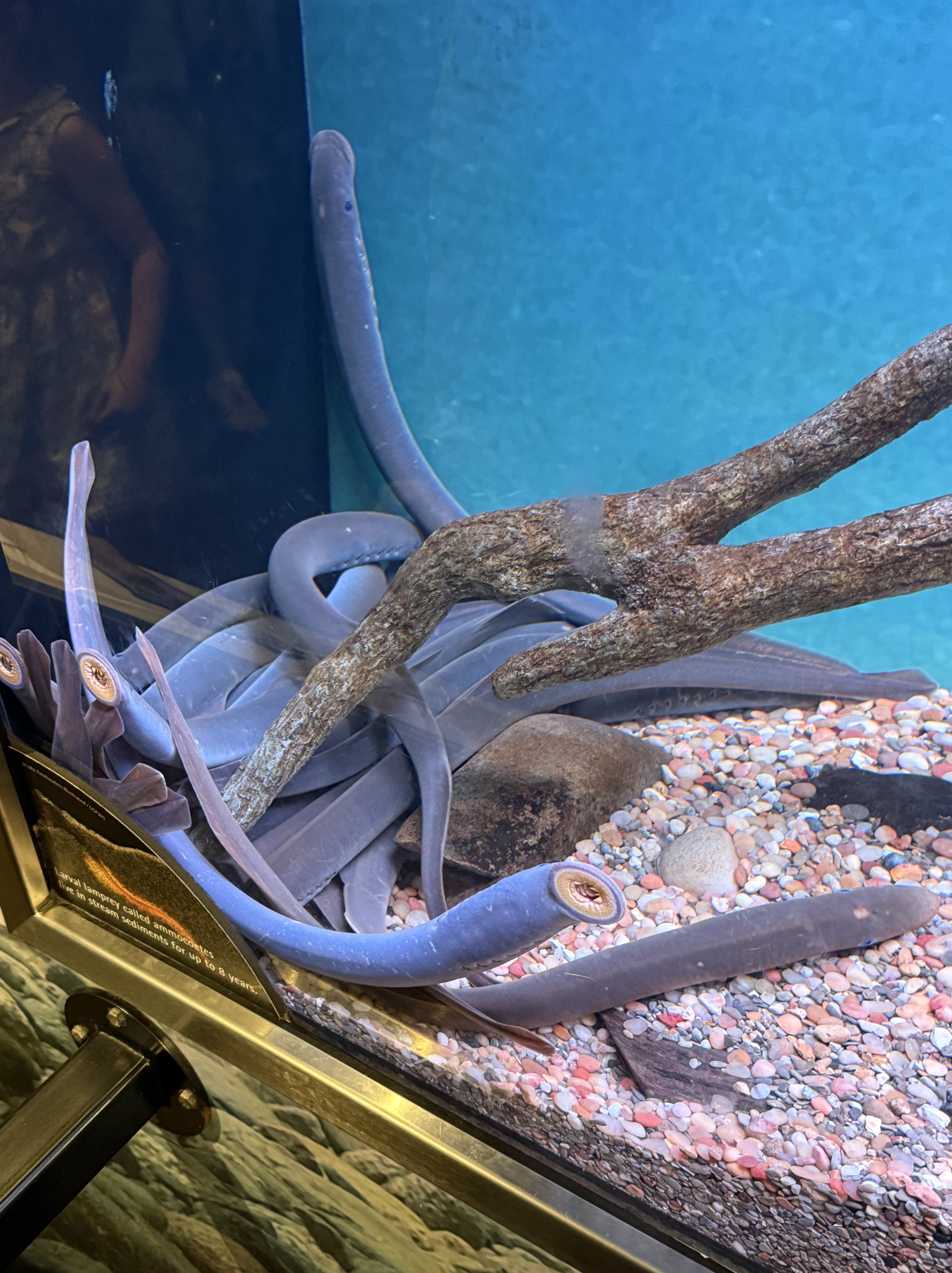
The lampreys were lying together in one end of a smallish tank. I guess it’s difficult to know whether they care about their surrounding or not. This is one strange fish.
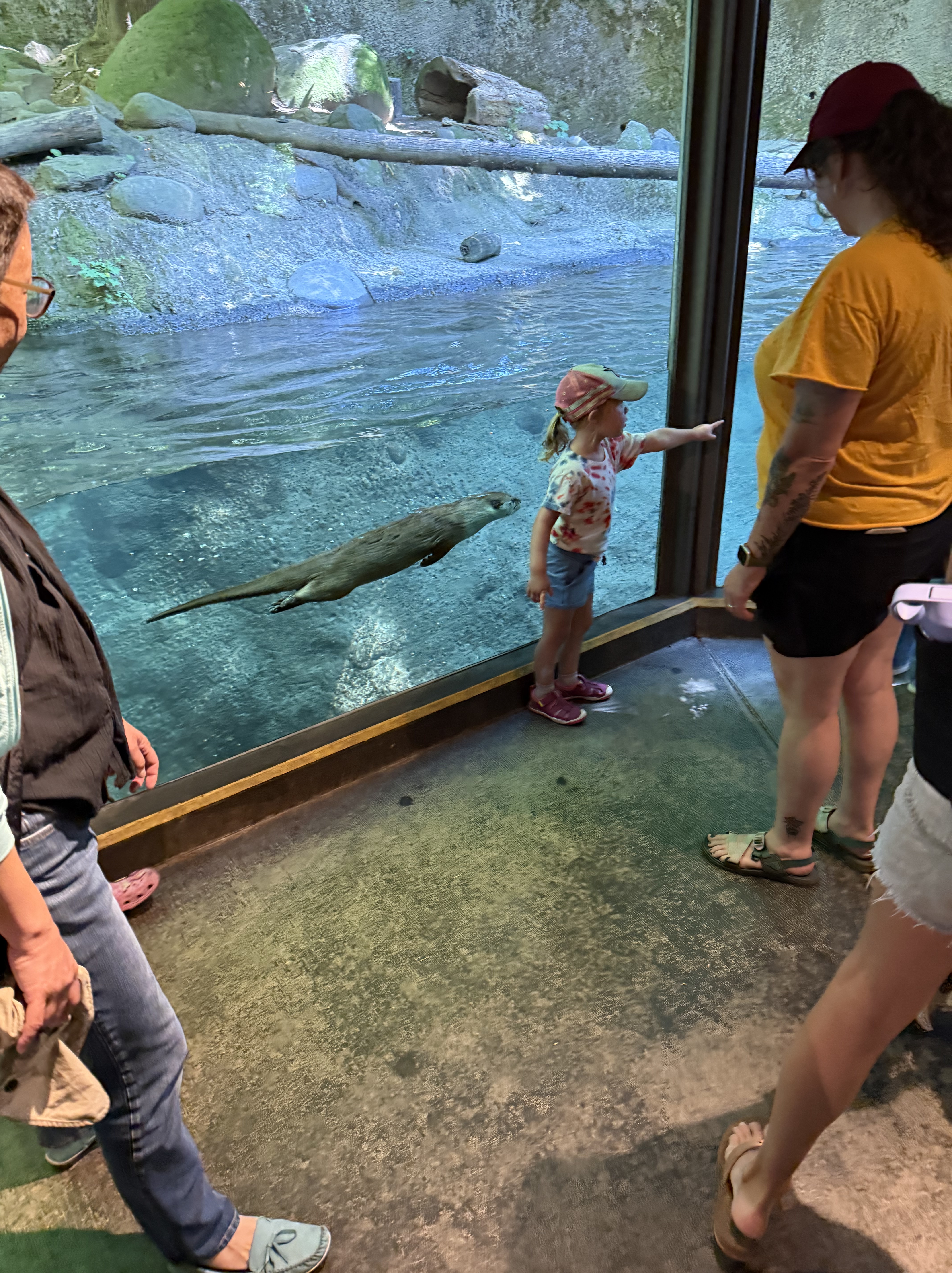
I never like to see free-wheeling animals like otters in captivity, even if they have cooled water to swim in. And I didn’t see any fish swimming around for them to catch. The phrase “feeding time” really bothers me, but I suppose we primates need to see the animals we share the world with in person to recognize them as being living beings. No one knows what an otter thinks…
This video shows a couple of otters cavorting in a viewing room. They had private places available, so I guess they don’t care if we reading monkeys watch them; but I wish that woman hadn’t kept her fat head so close to the window.
The mountain lion/cougar/etc is on the highest platform taking a nap, so I guess they’ve gotten used to life in a cage with a net ceiling. These big cats, native to all of N. America, aren’t endangered, but, obviously, we can’t see them this close. They are pretty dangerous.
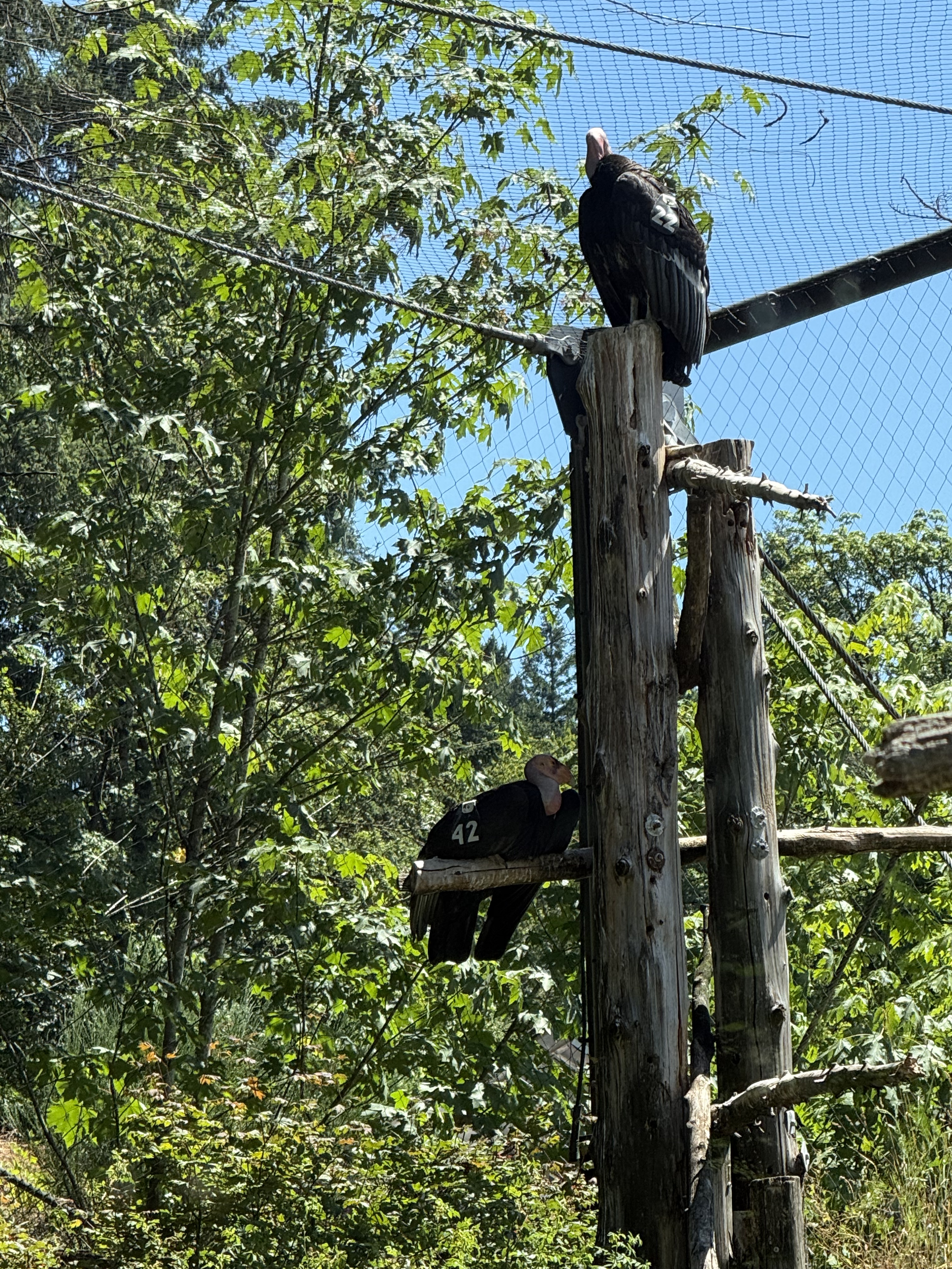
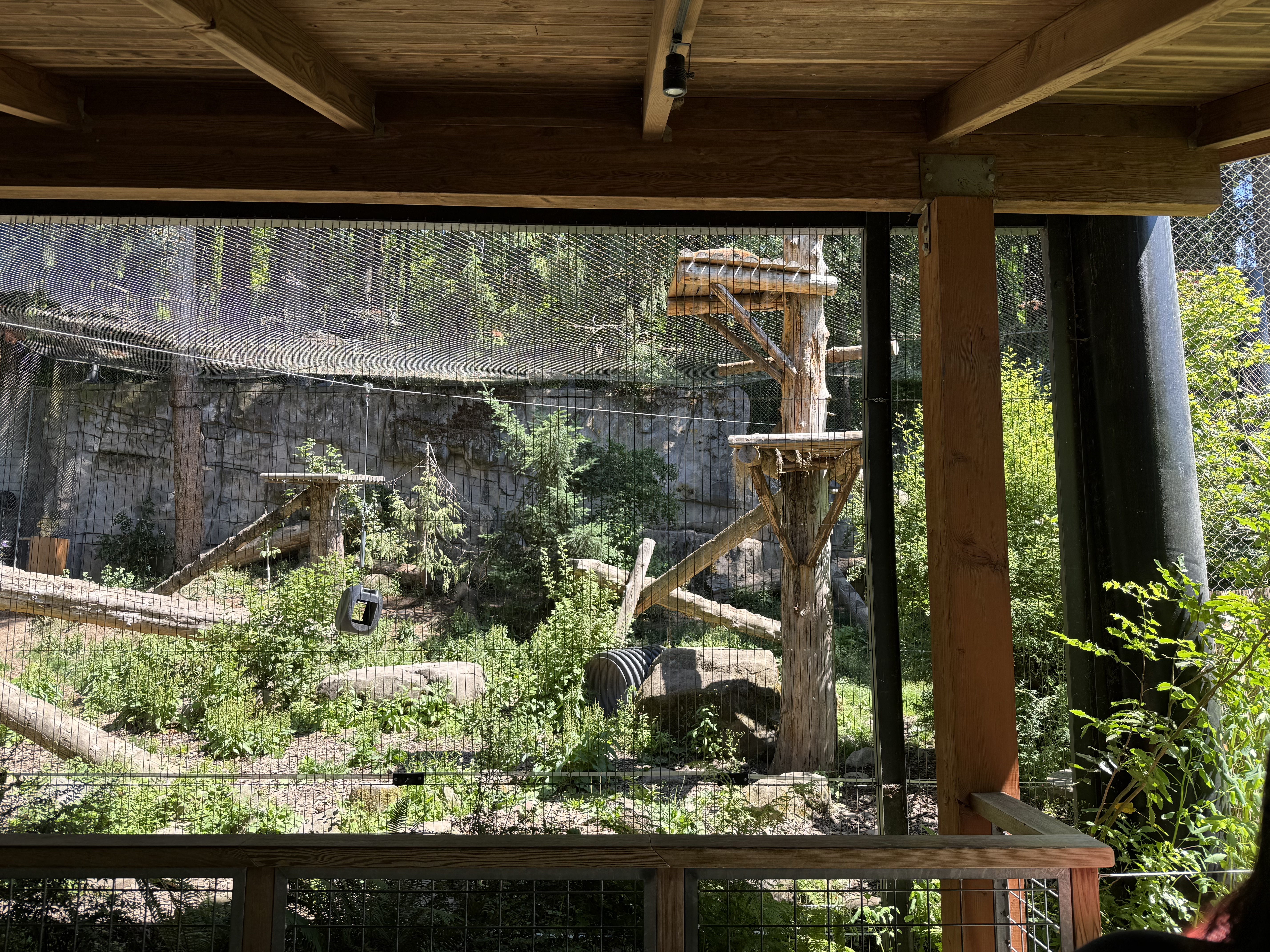
I was feeling pretty bleak about the whole zoo concept until I saw the condors. They were actually EXTINCT in the wild until the efforts of zoos reintroduced them; now they are coming back, each one wearing a team number and a radio transmitter. I guess this is their “halfway house” before winning their freedom.
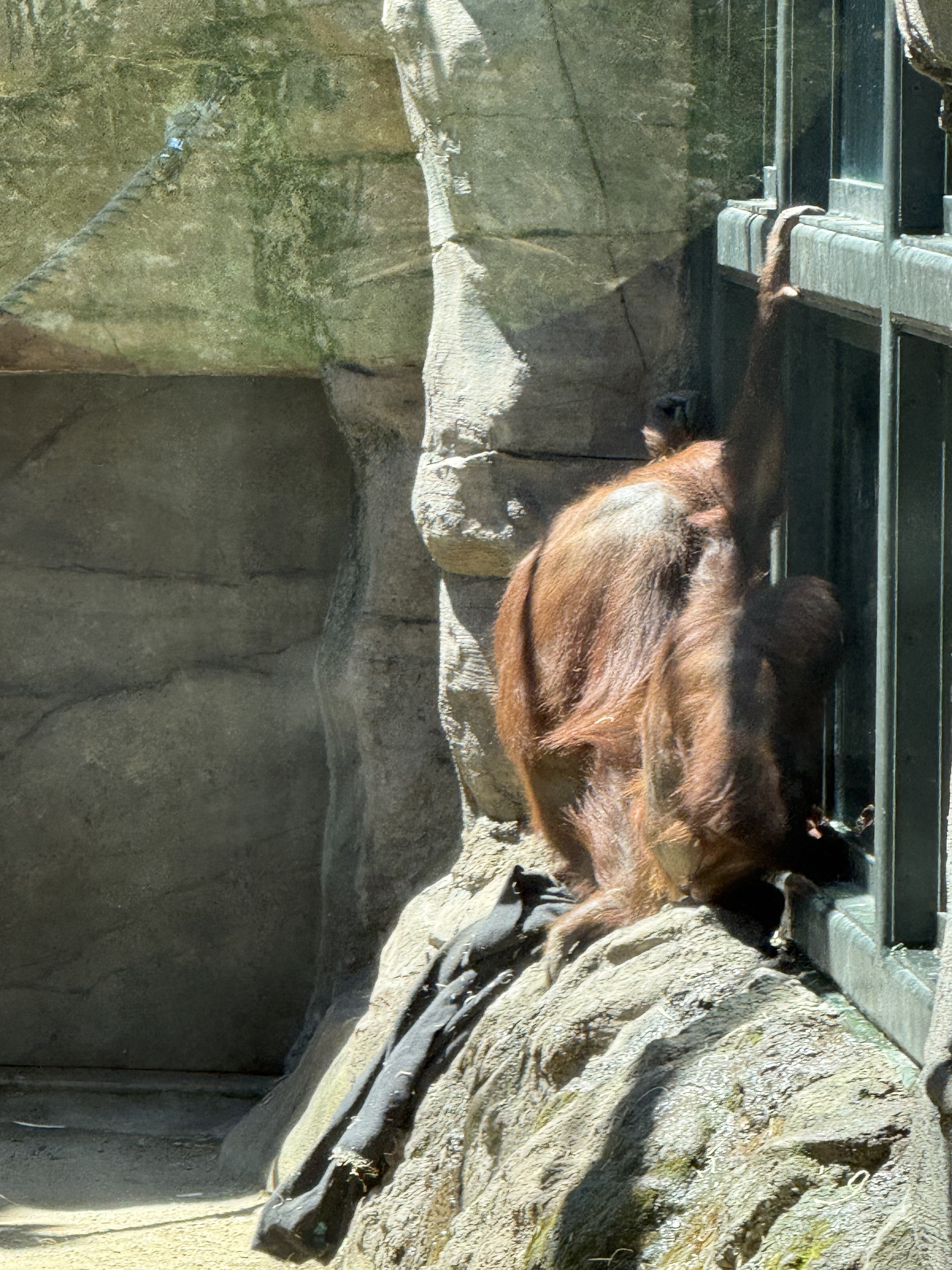
The primates have a series of habitats. Unlike some of the other prisoners, they take an interest in their captors’ antics; these orangutans are watching their human helper clean their bedding (airing and replacing straw). The looking glass works both ways…
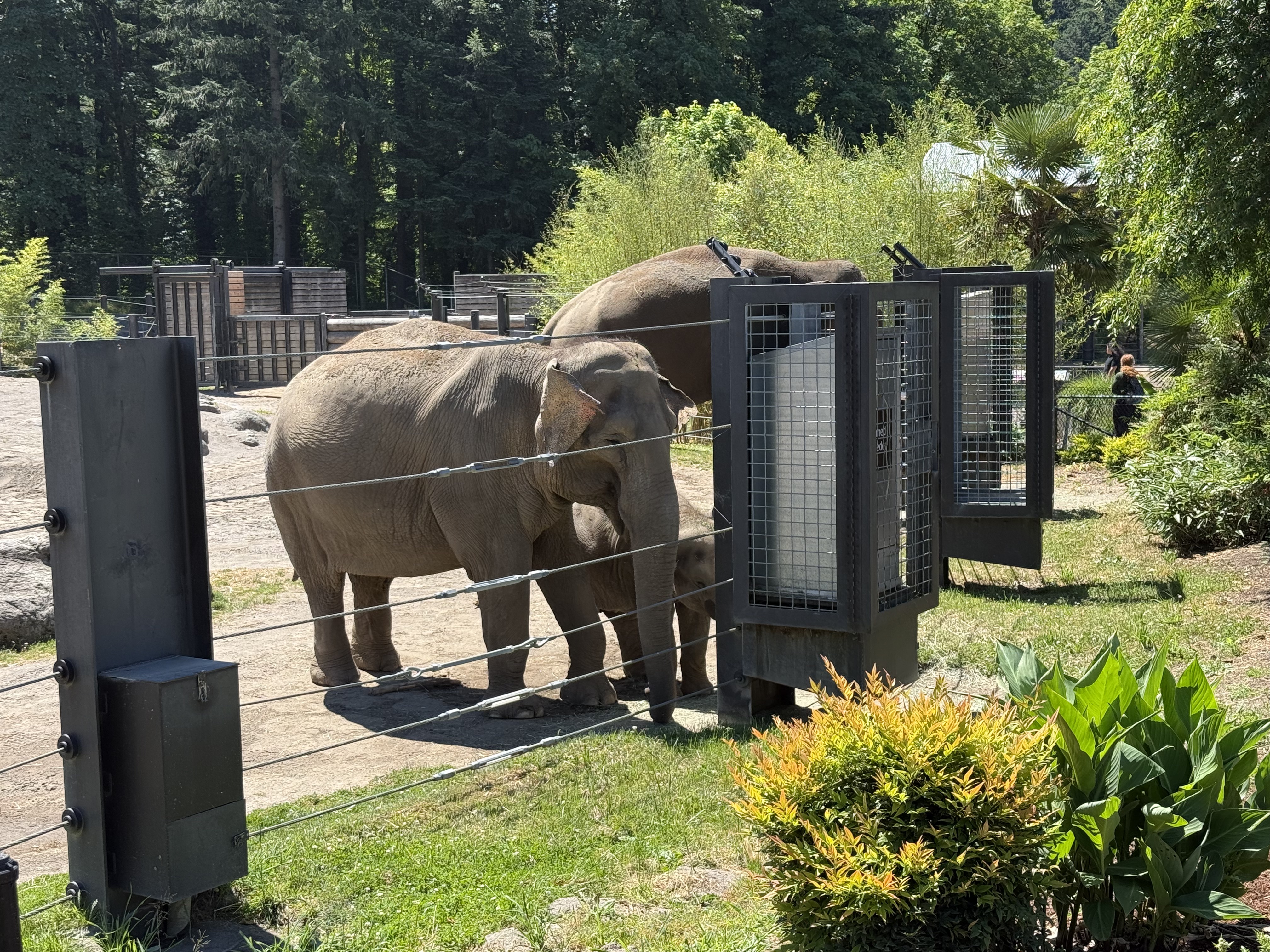
The zoo has named their “guests” because they are trying to support social systems like these elephants would have in the wild. Thus they have family groups (even in animals that don’t have “nuclear” families). For example, one of the males was in a sexually provocative state and isolated in the enclosure seen in the background so that he couldn’t fight with the other males, or injure the young one; but another who was considered “safe” was mixing with the “herd” while feeding in a separate “males only” trough until…
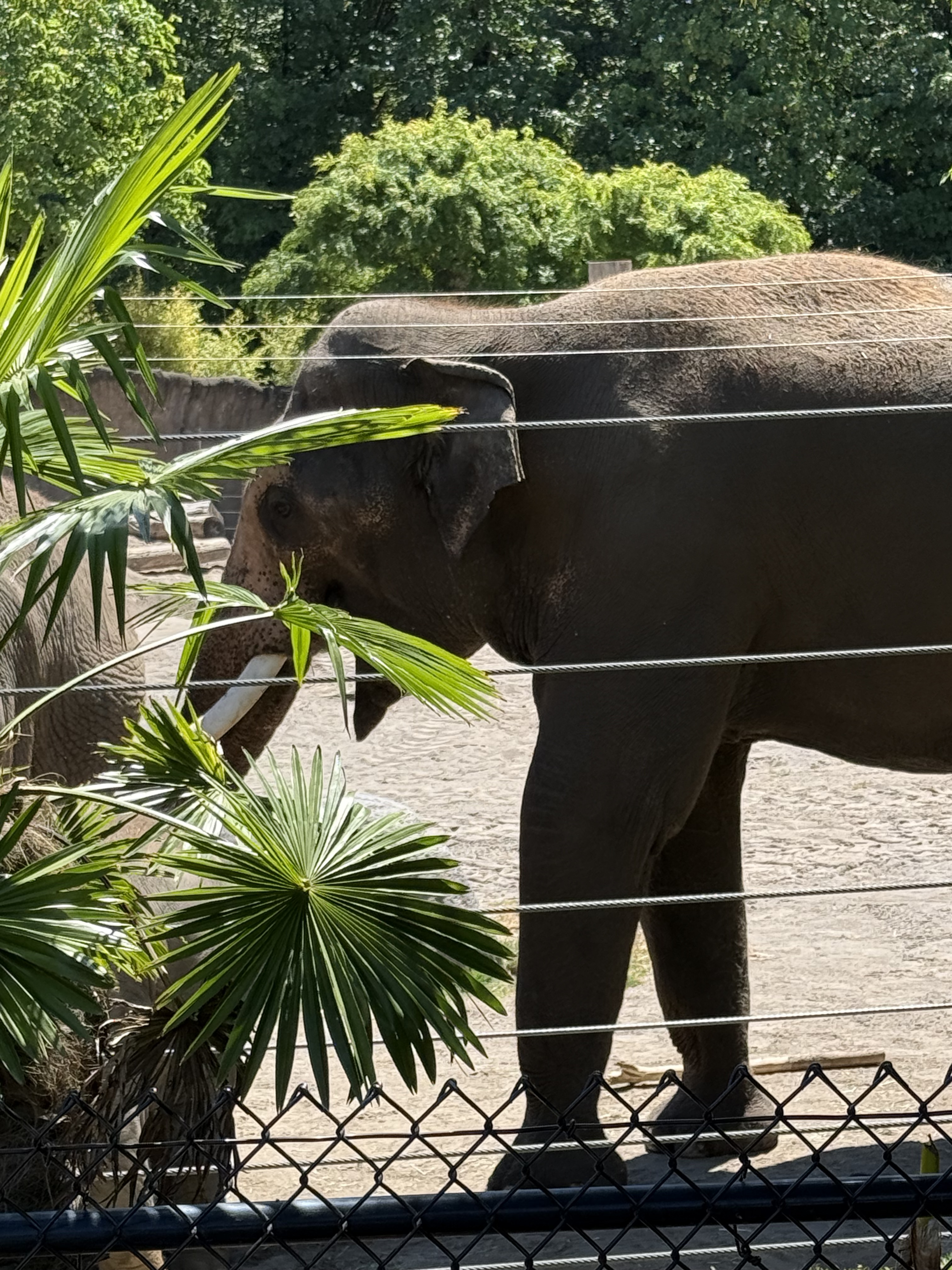
He finished his plate and pushed the others, including the young one, aside to eat their food. These large animals really need many square miles to live. This situation is like having your entire family living in a studio apartment, which people do in some parts of the world; nevertheless, elephants are at the top of my list for animals that will be eradicated by humans because they simply require so much SPACE to live, and they consume massive amounts of resources. I hope they don’t follow the path of the condors, and I applaud efforts like these–hope for the best but prepare for the worst-case scenario…
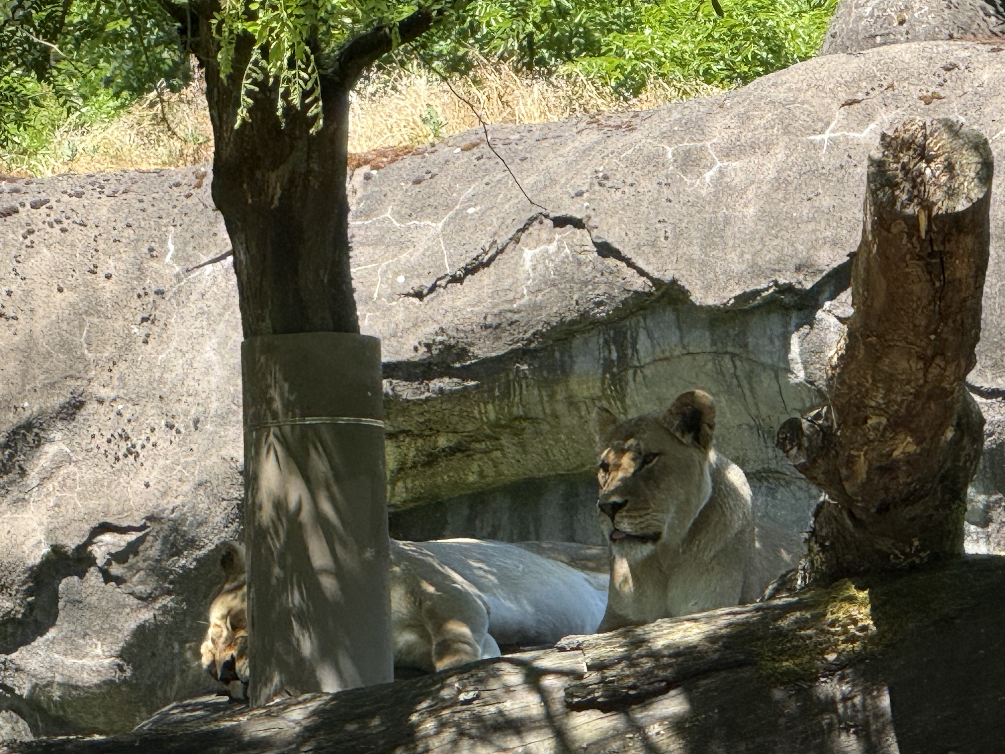
I could barely see these lions, but my phone’s camera caught this image. Words fail me to describe what might be going through this loin’s mind…
These lemurs don’t seem to care that a bunch of primates are watching them as they wake from a nap…
This monitor’s tail is half as long as its enclosure. A photo can’t convey its situation as well as a video, even thought it isn’t doing anything dramatic, but–what is it thinking? I have no idea; maybe it is perfectly happy–well fed, as cool or warm as it desires…
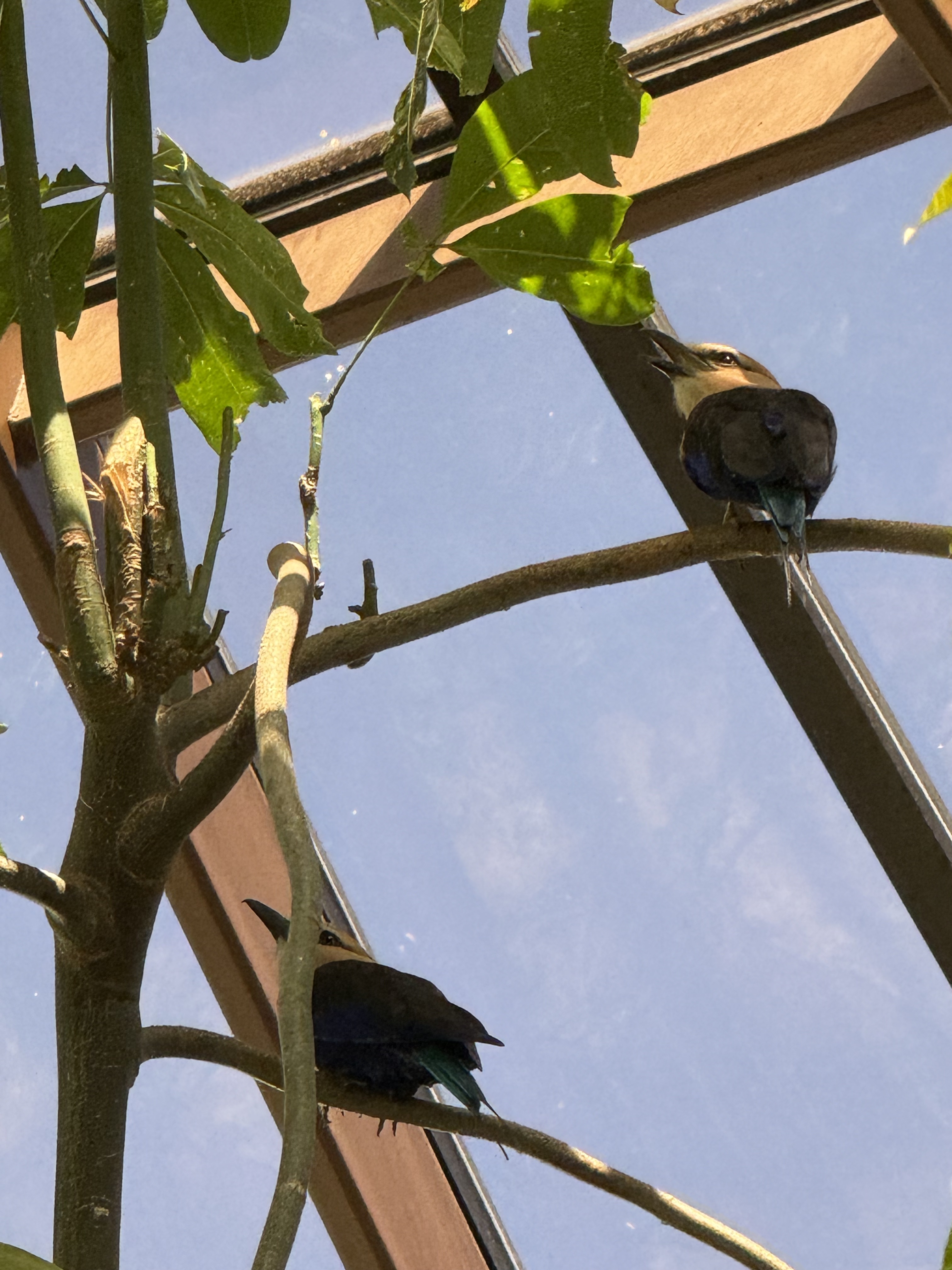
There were a lot of birds in the bird enclosure–small ones that could fly around, larger, flightless ones that hung around the door as if waiting for a chance to escape.
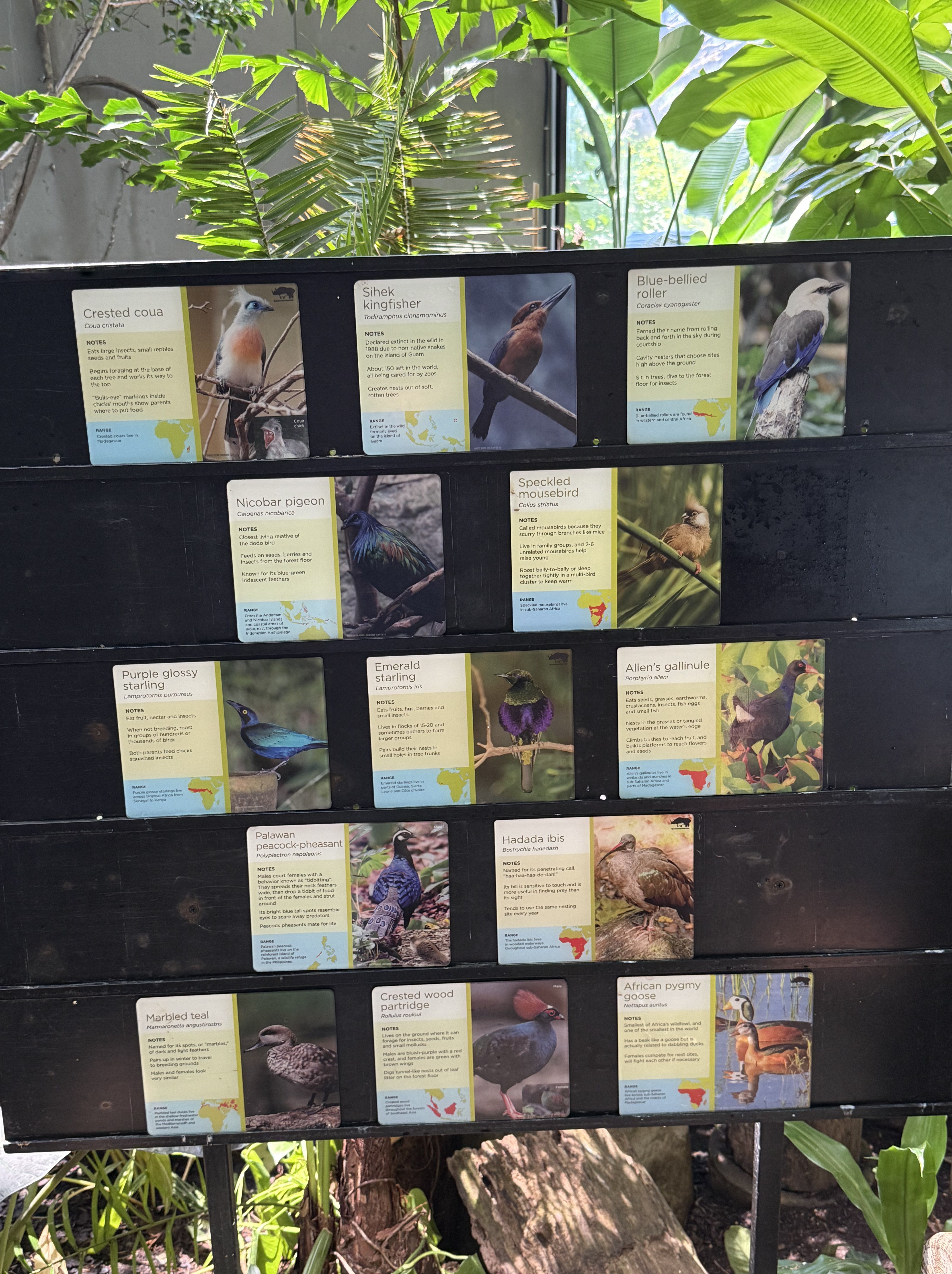
I saw several of these, but they didn’t pose for photos. None of them looks like the birds from the previous photo, but I don’t know anything about birds. Maybe the listing is out of date…or maybe I’m a typical modern Homo sapiens, who is so unaware of the physical world that…
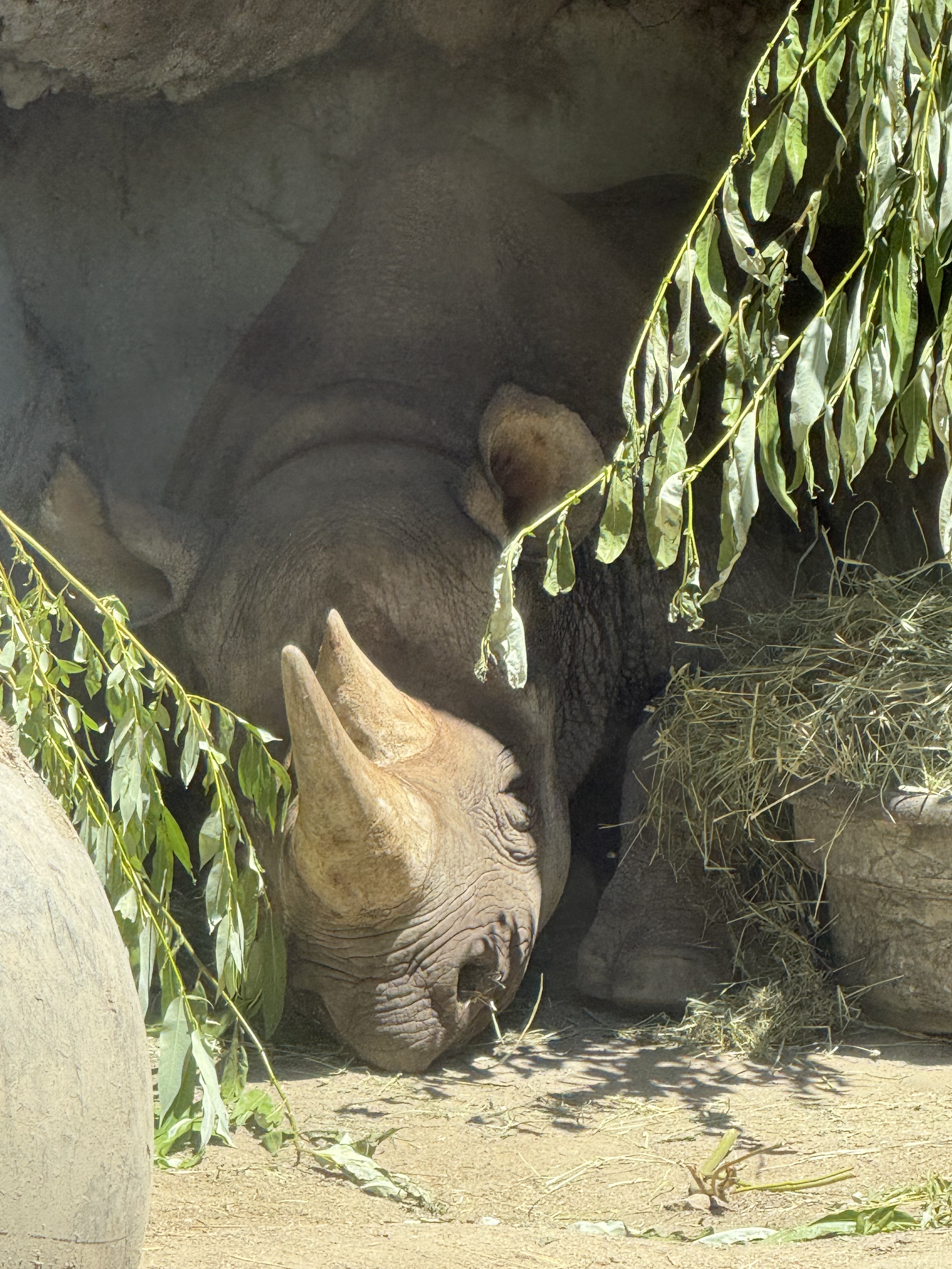
Thank god my phone could see in extreme contrast. I never saw this rhinoceros lying in the shade, apparently listening to every word we primates were saying. This is another example of an animal that requires a lot of SPACE to live; the Oregon Zoo did its best with what was available, even creating a “family” environment with several animals living together.
This tiger doesn’t say much, but their stately demeanor says more than words…
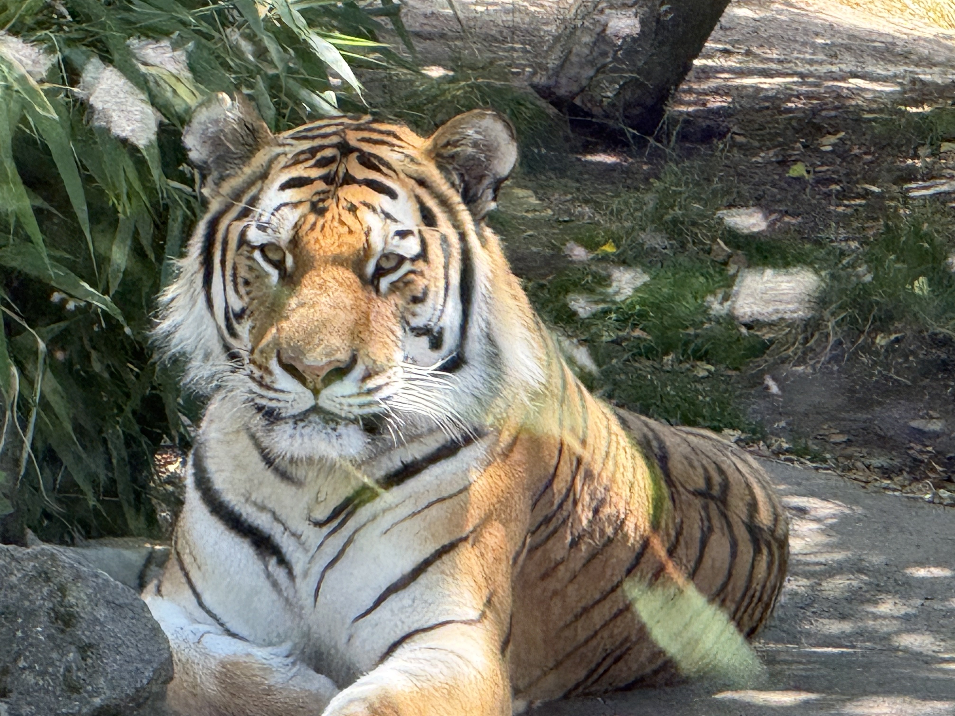
I got this image without seeing what I was photographing. With the light/shade contrast, I was blind but my camera wasn’t. What is this magnificent creature’s expression conveying?
I try not to anthropomorphize because none of the animals held captive in the Oregon Zoo are human. They aren’t stupid, intelligent, emotional, sociopathic, or anything else we sapiens self-classify ourselves as. They are simply not in a position to influence the physical world as dramatically as we. Lions and tigers don’t create cages to hold their prey before they become a meal. They hunt when they are hungry and eat what they can catch.
I don’t think my feelings about zoos have changed after my visit to this excellent repository of the animal world. Nevertheless I understand the conflict between humanity’s claim to dominance, as the top global predator, and the responsibility that comes with this natural order; what I mean is that we are the children of Earth, just as is the tiger and the bacteria. However, with great power comes great responsibility, and it is incumbent on us to accept the difficult challenge of preserving life to the extent of our abilities.
Every animal I saw in the Oregon Zoo is, or will soon be, threatened by humans. Maybe we are the cause of the next great extinction–if so, such an ominous responsibility should be treated with great circumspection. This is no light matter.
Whether we like it or not, we are responsible for the fate of life on Earth…
A Day Trip to Yakima
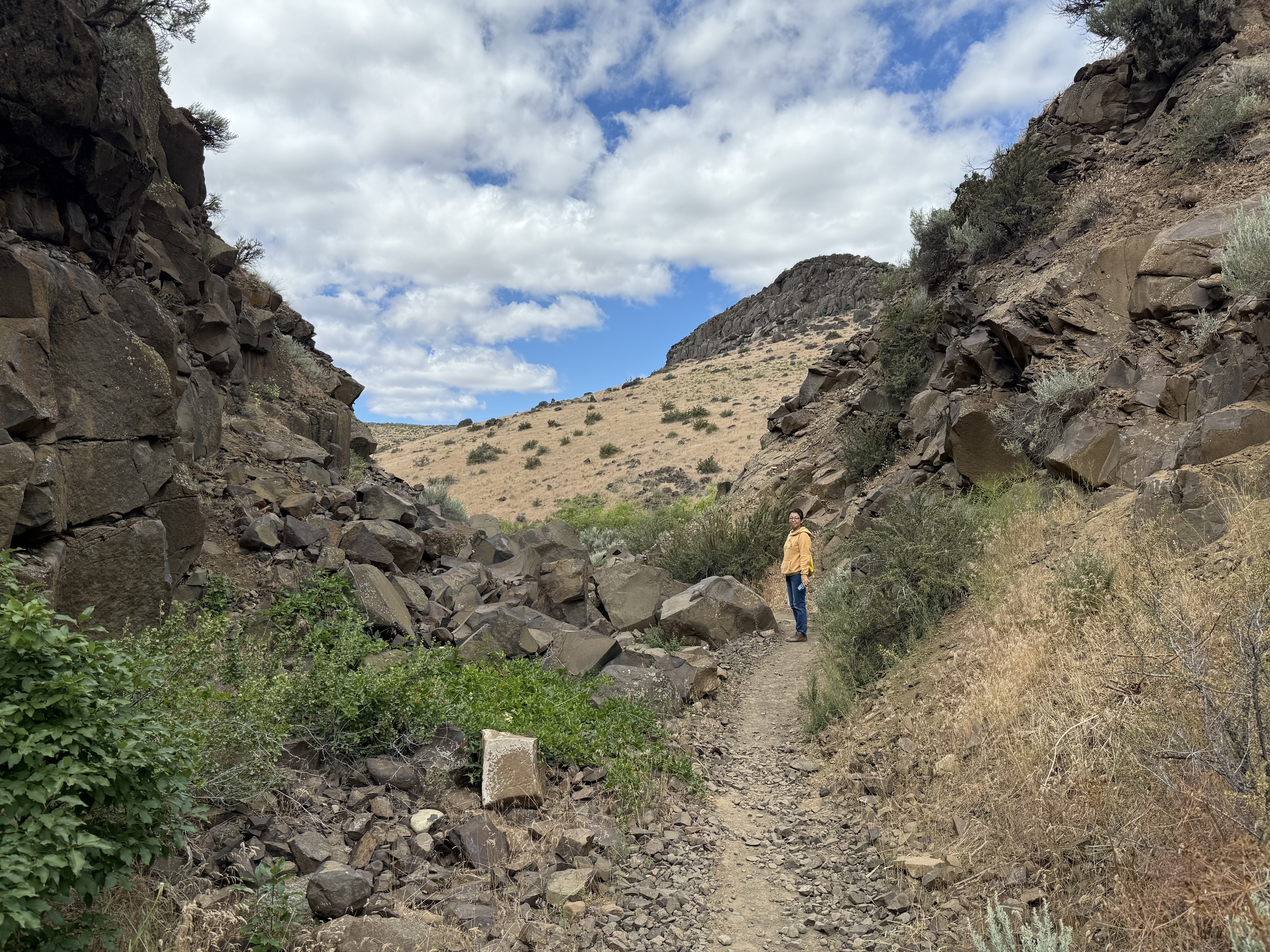
We wanted to see what was on the other side of the mountain, so we headed east from Tacoma and crested the Cascades at Chinook Pass. It was snowing at the pass and fog/clouds obscured what were probably majestic views. We pushed on to Yakima and found the Cowiche Canyon recreation and conservancy area.
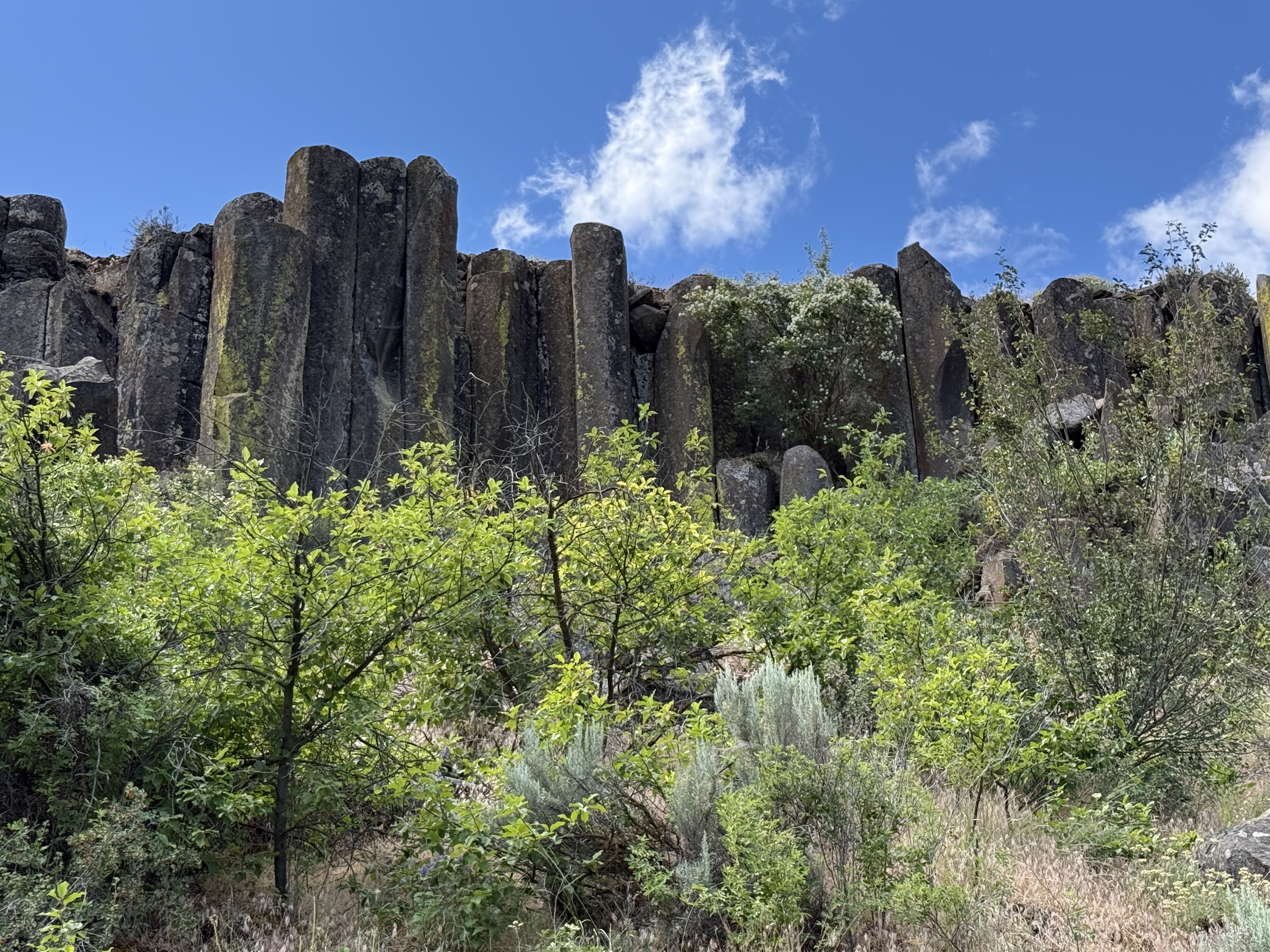
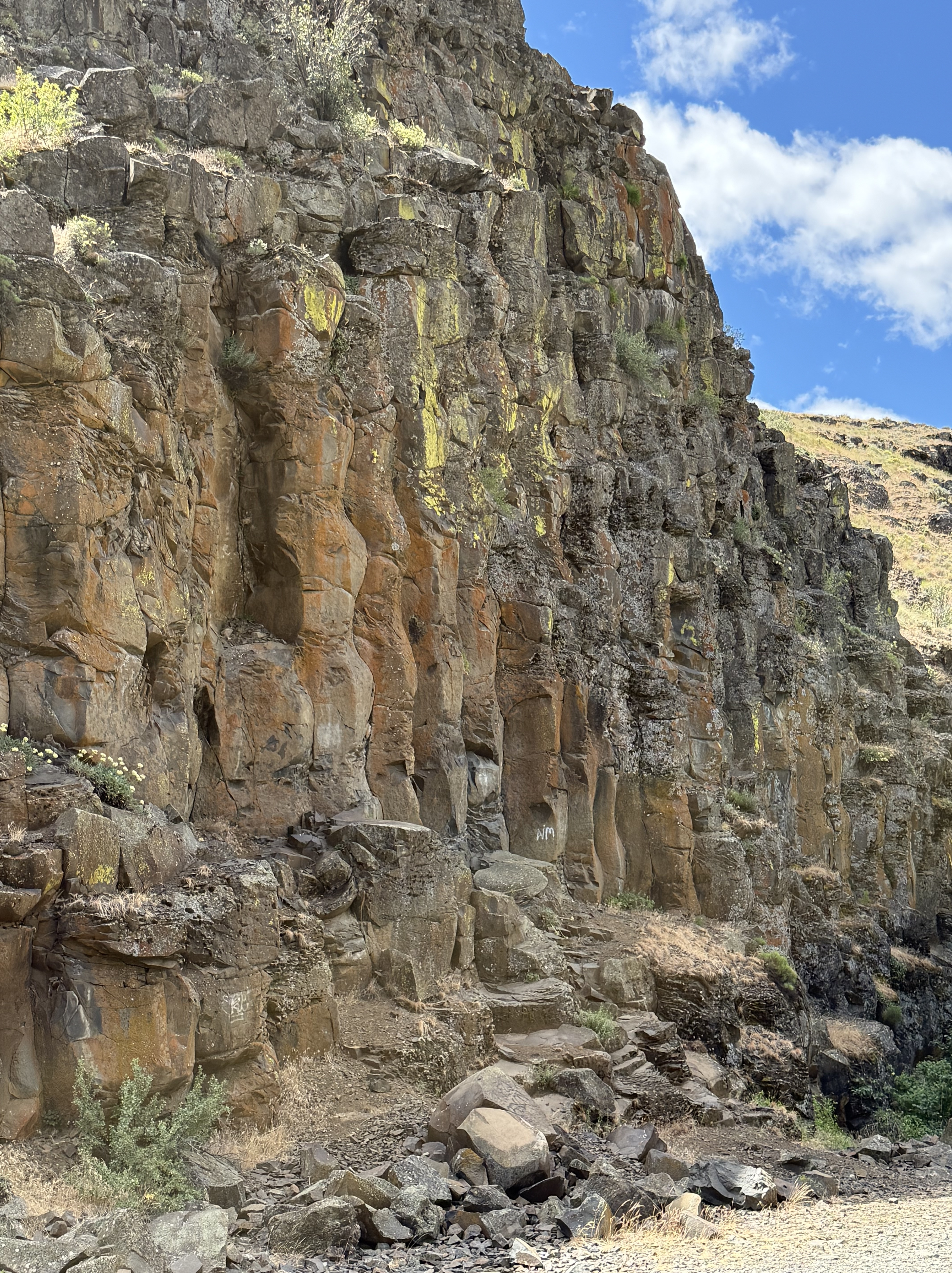
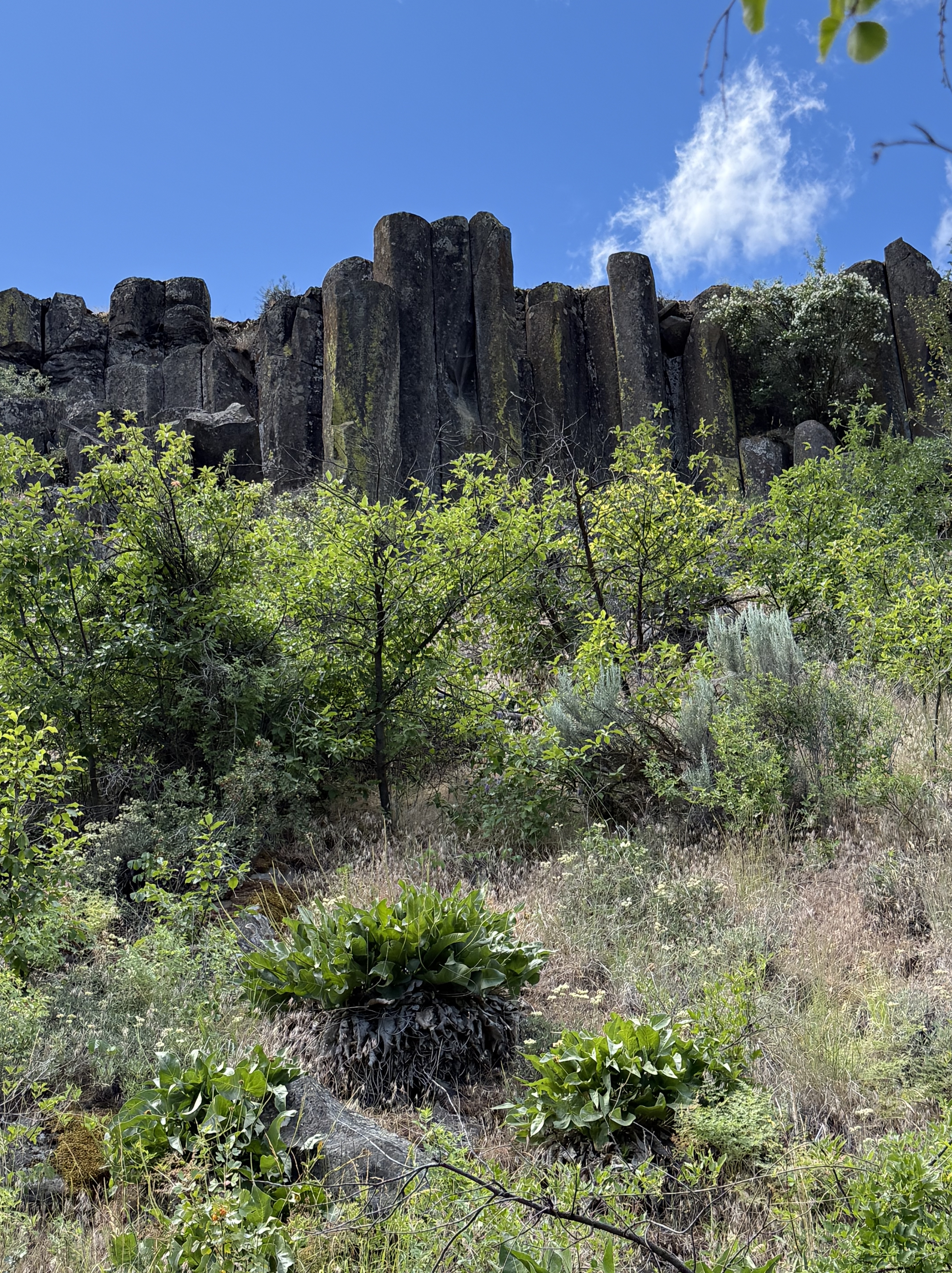
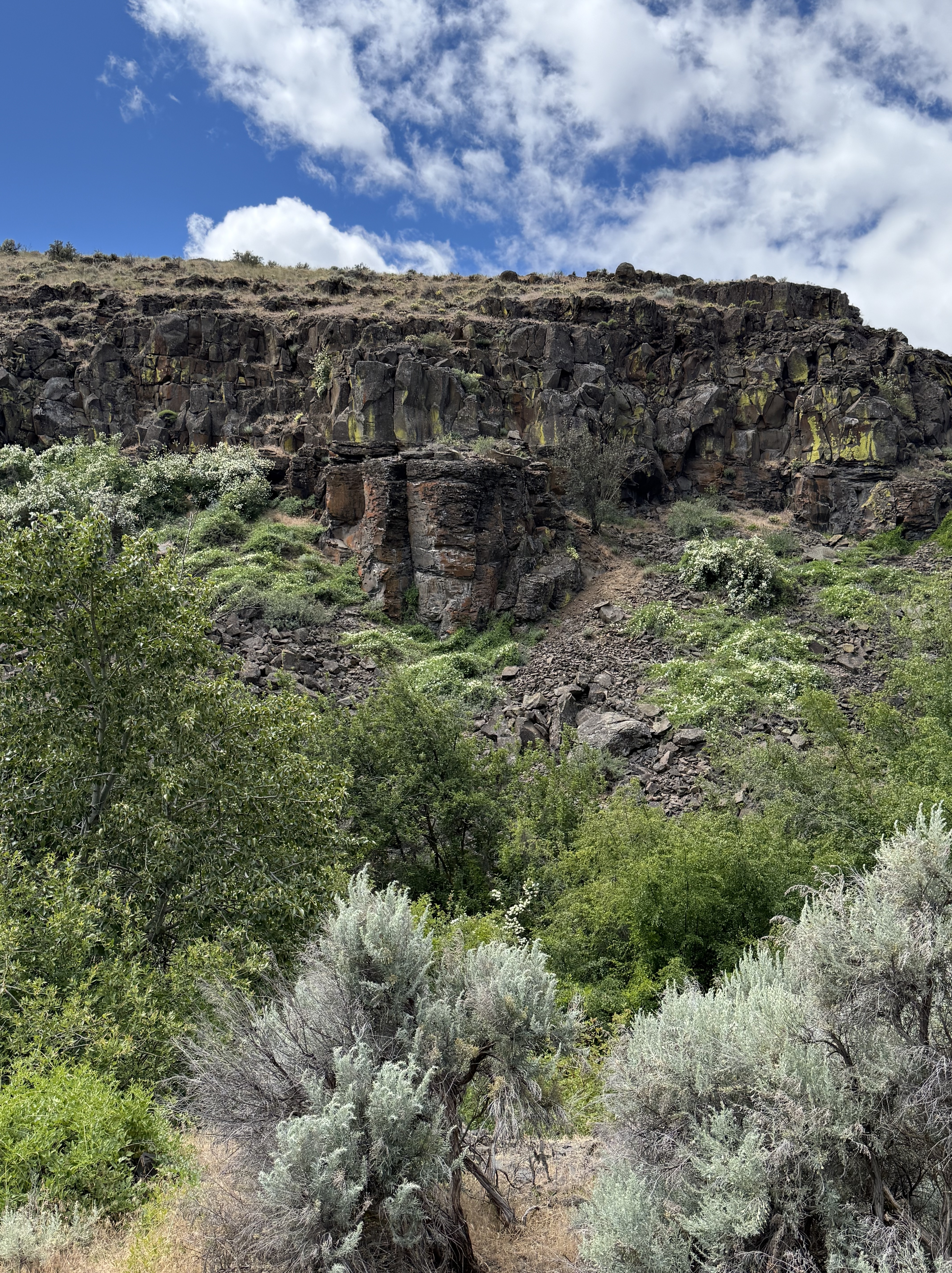
This is a typical view from the trail, which follows an old rail line that was used for seventy years to haul apples out of the area. I have discussed the columnar basalts and vegetation in previous posts. It was late spring and all of the plants were showing their color while water rushed past in the creek at the bottom of the canyon.
This undulating columnar basalt caught my eye because of the color and its wavy appearance.
The Burlington Northern railroad wasn’t afraid to use explosives to create a path through what was described at the time as, “A dry, rocky canyon good for nothing except a railroad.” The rails have been removed, but the eleven bridges required to construct a rail line to cover the 3 miles of the trail system are mostly still in place.
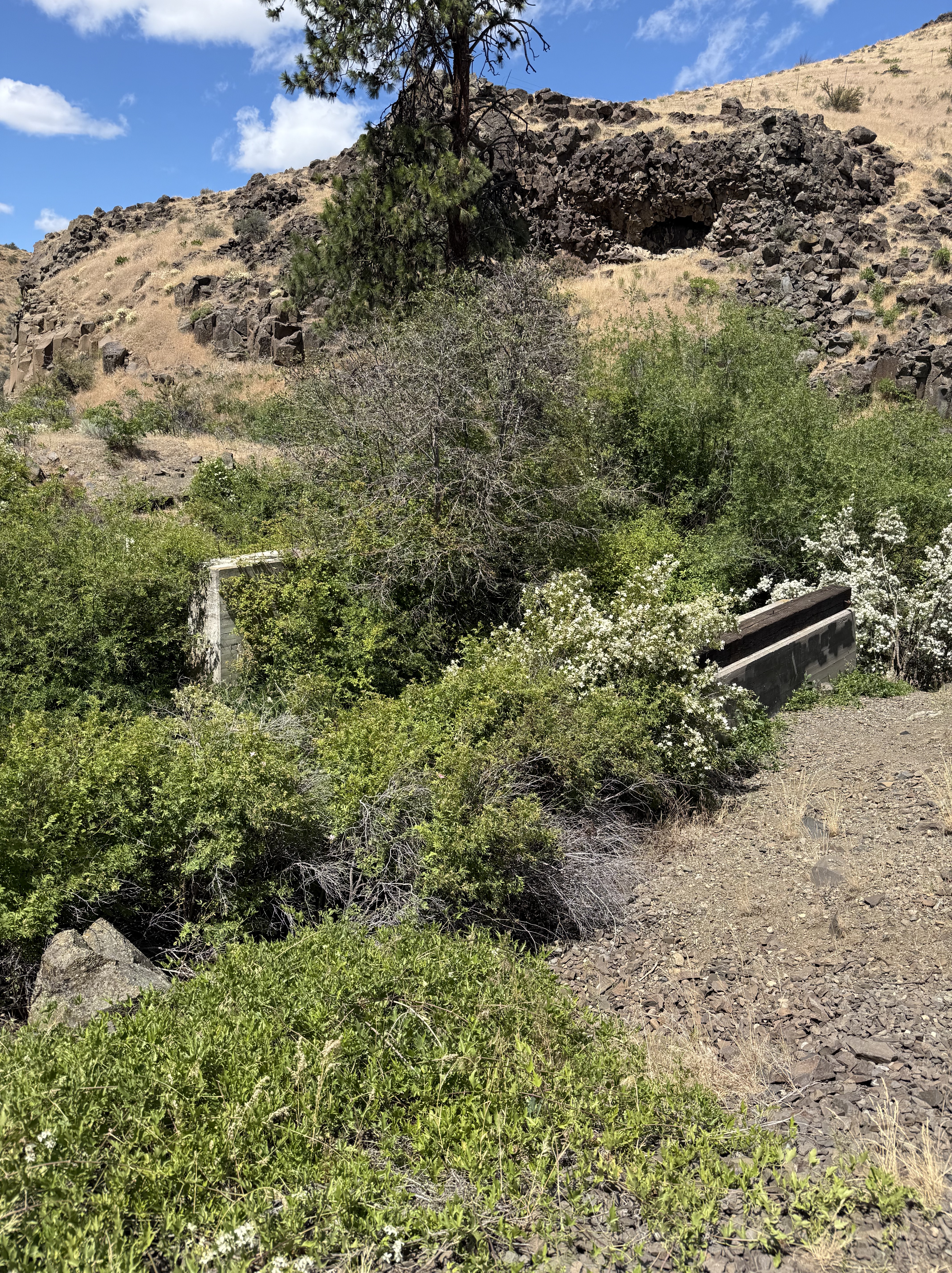
Here’s one that didn’t last. It was replaced by a pedestrian bridge constructed by the Cowiche Canyon Conservancy and the Bureau of Land Management.
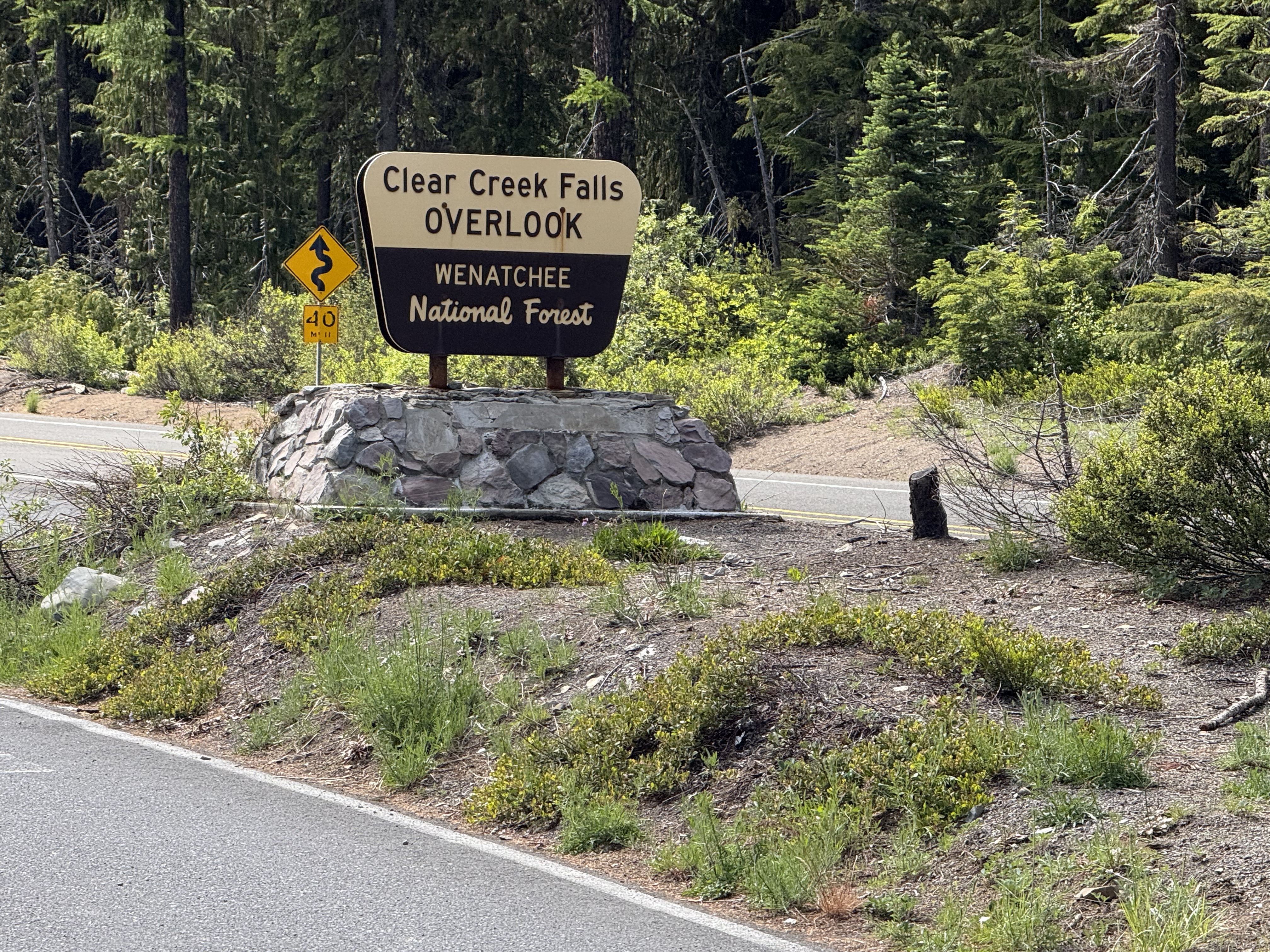
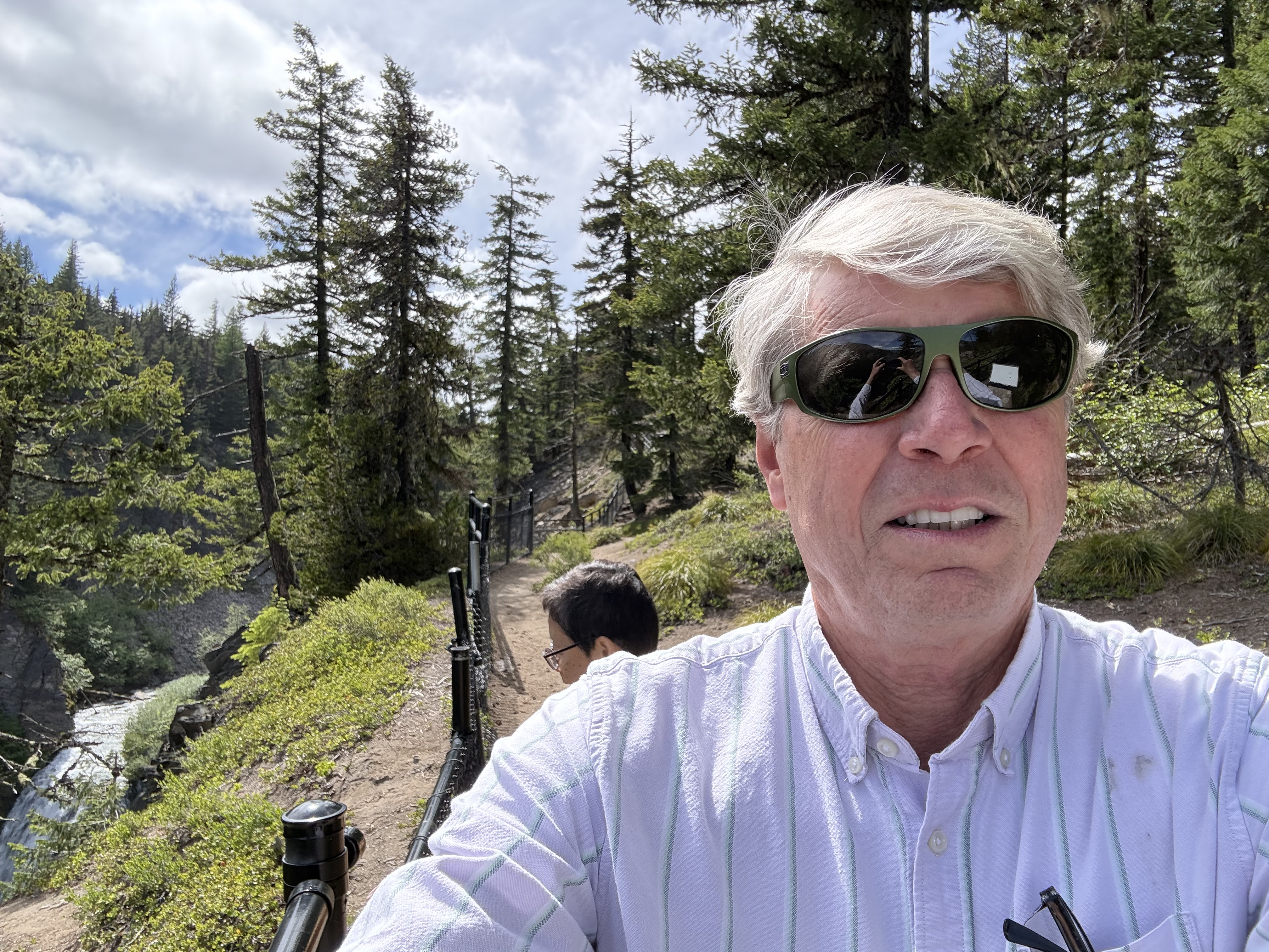
We took a more circuitous route back to Tacoma using US12 through White Pass. It didn’t snow, and we got a look of one of the many water falls in Washington.
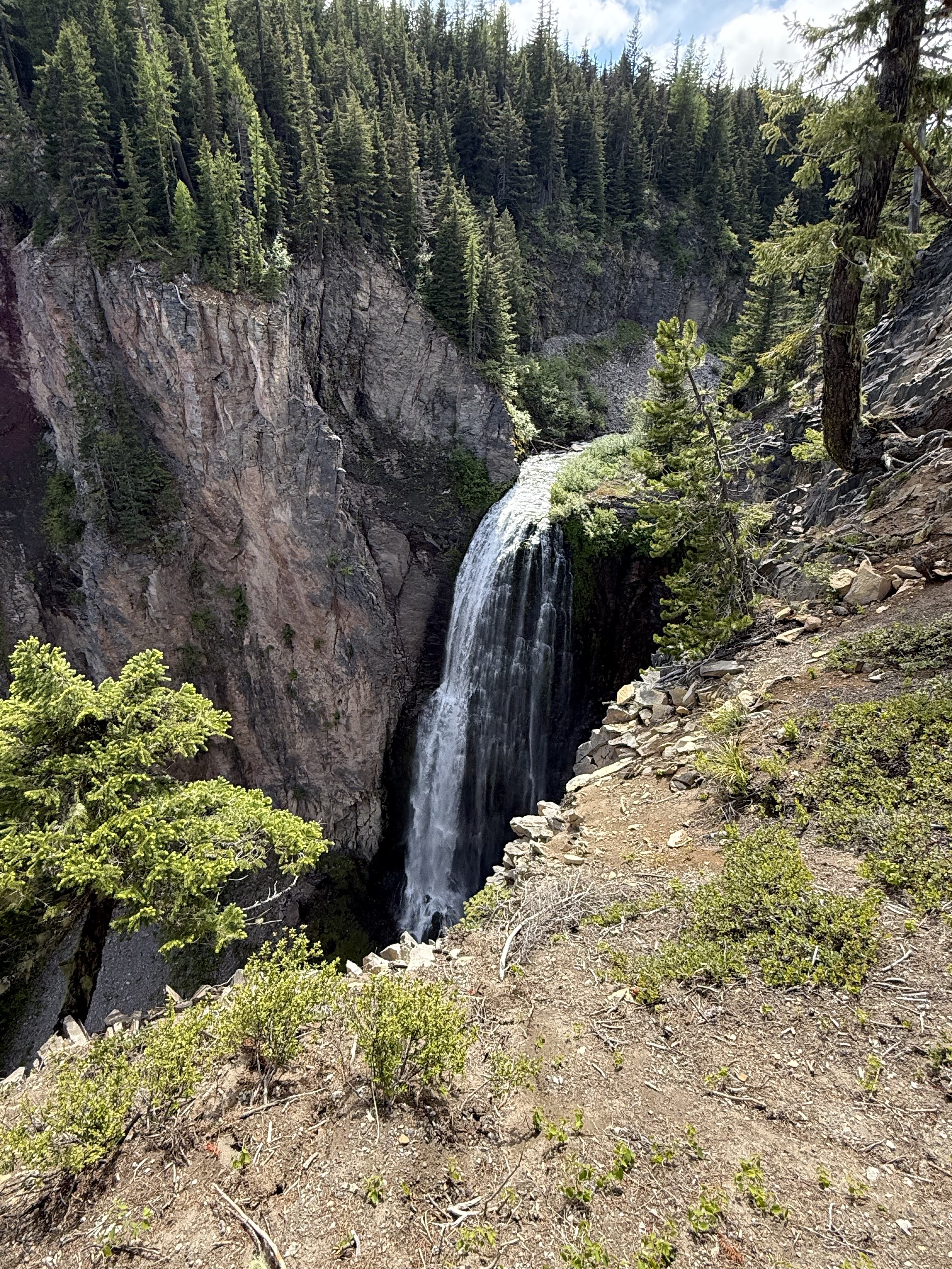
This was the best angle I could get, and I still couldn’t see the bottom! It turns out that Washington has more than 3000 catalogued water falls, more than any other U.S. state. Clear Creek is rather small at only 300 feet, so I guess there is some more air down there.
It was a beautiful day in the Pacific Northwest, including the snow flurries. A ten-hour day trip took us from coastal Washington, over a 6000 foot pass, into dry eastern Washington, where we hiked through a canyon filled with native plants and rocks (hahaha), and back over the Cascades past a magnificent water fall in Wenatchee National Forest.
This is undoubtedly the most beautiful place I have ever lived…
Ecological Notes from Cowiche Canyon
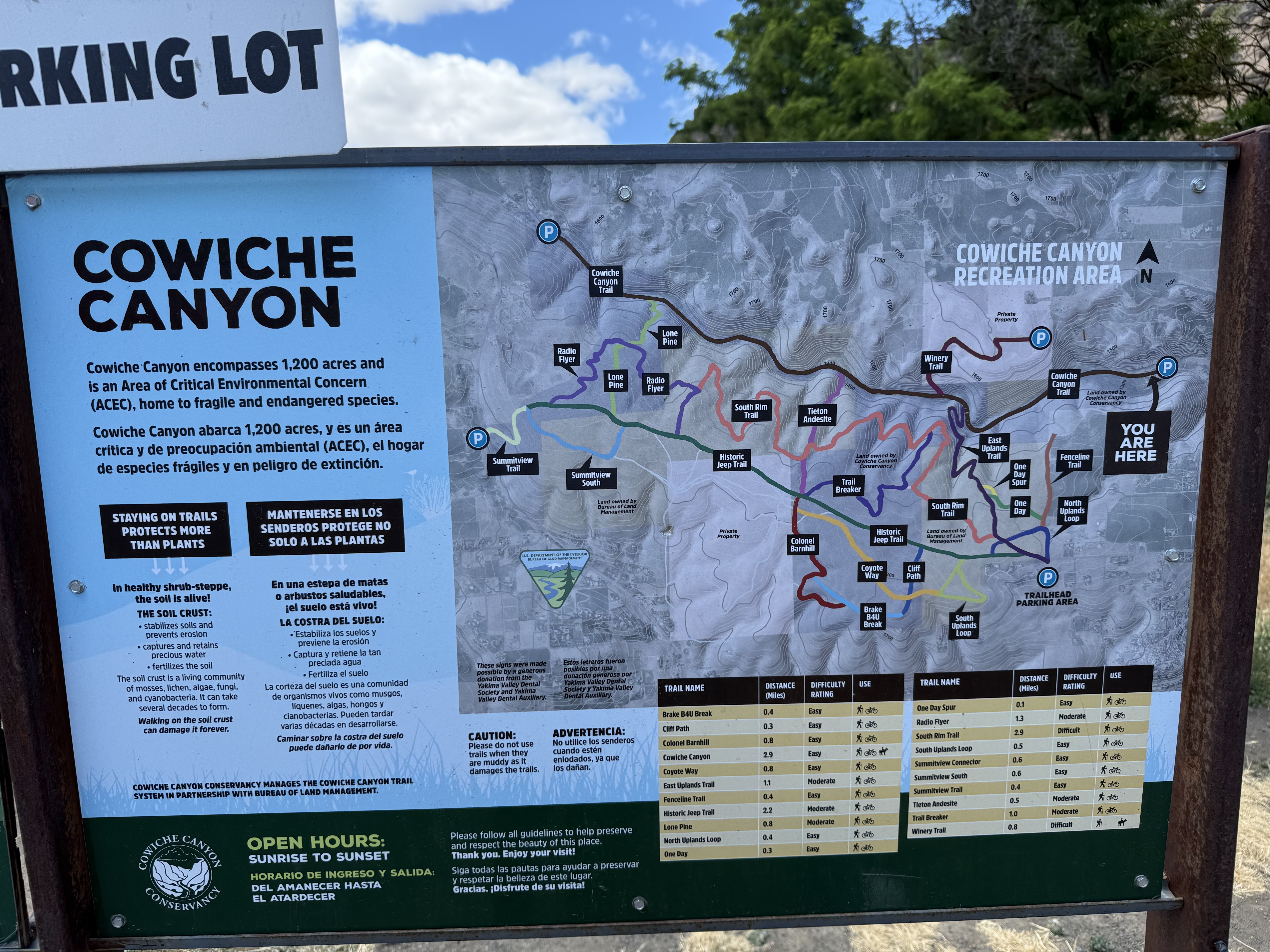
Cowiche Canyon Recreation Area is located on US12 just west of Yakima, Washington. The region receives 9-14 inches of rain per year, making it a dry area; thus, the trail system includes both shrub steppe (uplands) and riparian (along Cowiche Creek) habitats. We followed the main trail along the path of a rail line that was in use between 1913 and 1984 along the creek; however, the wetland is very narrow, in places constricted to less than 100 yards. Thus, I encountered plants from both environments.
The canyon walls are composed of a series of basalt ledges with intervening slopes covered by talus and colluvium, which are part of the shrub-steppe habitat. I discussed the geology of the area in another post.
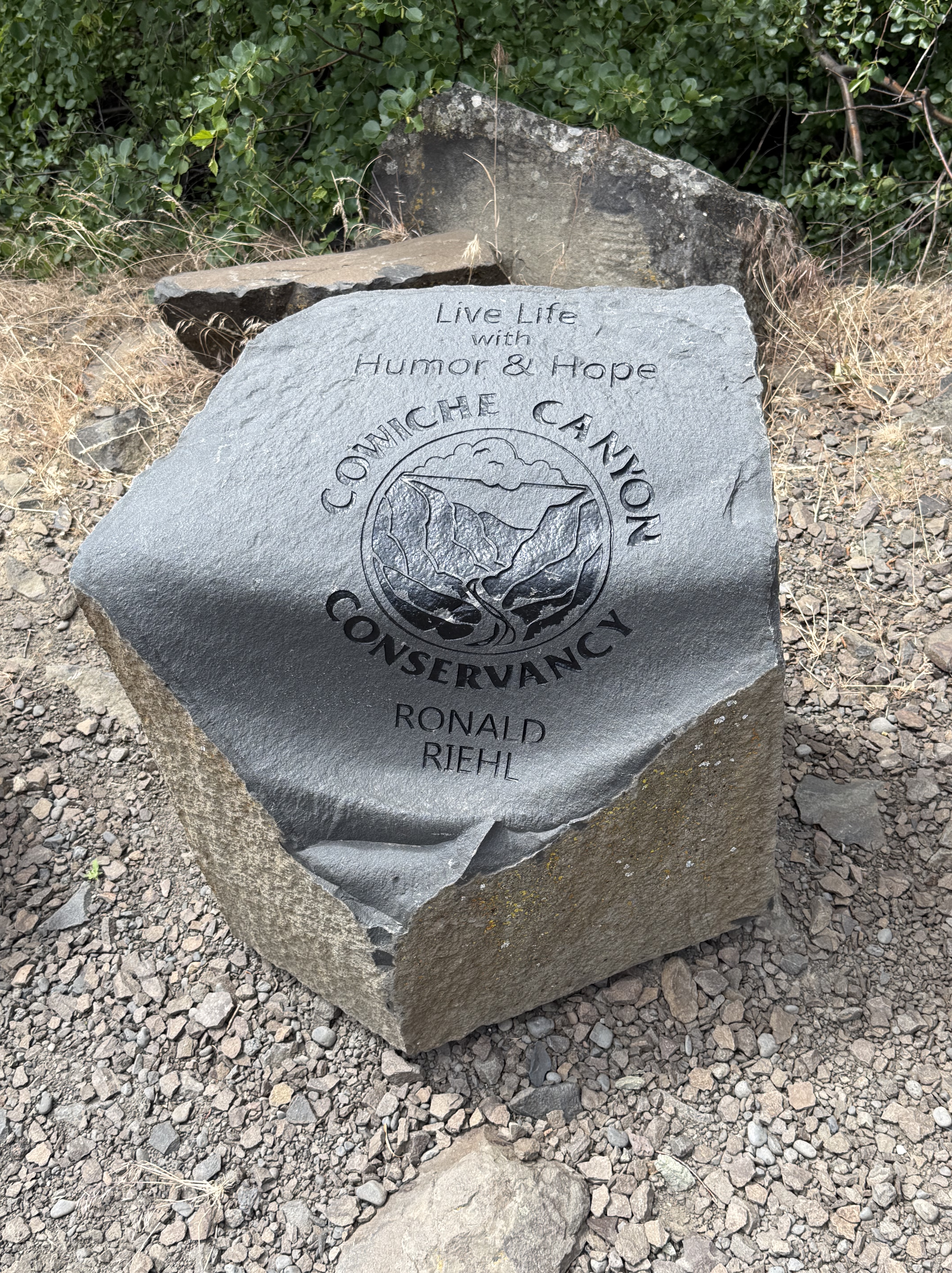
The recreation area is maintained by the Cowiche Canyon Conservancy in partnership with Bureau of Land Management. This stone is a piece of the columnar basalt that lines the canyon.
It’s fortunate that I visited this area during spring, which lasts a little longer here in the Pacific Northwest. As always, I used CoPilot (AKA ChatGPT) for identification while I try to remember scraps of the huge amount of information presented in this mixed environment.
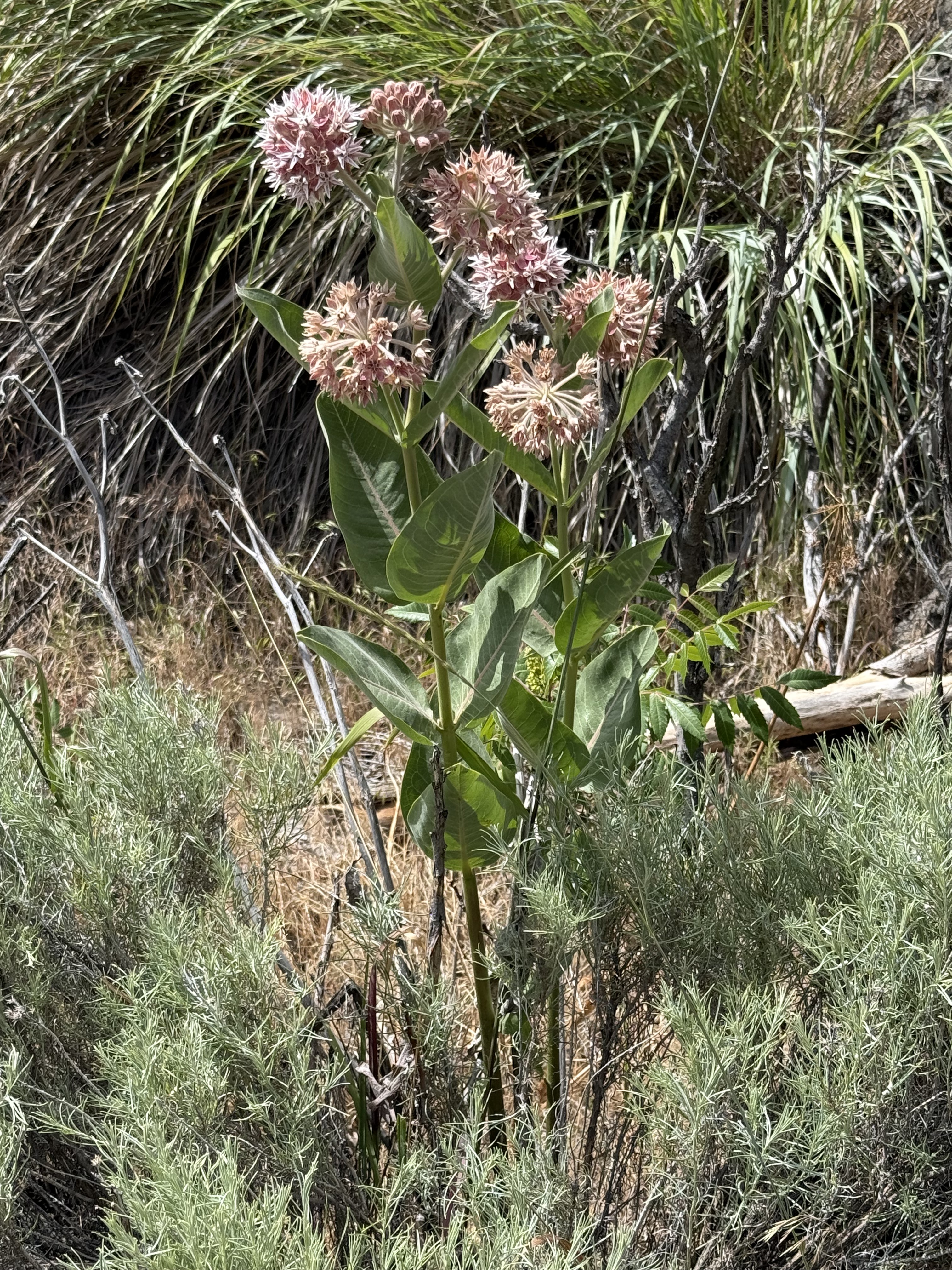
This is Asclepias speciosa, also known as showy milkweed. It is native to Yakima county and is a host species for Monarch butterflies.
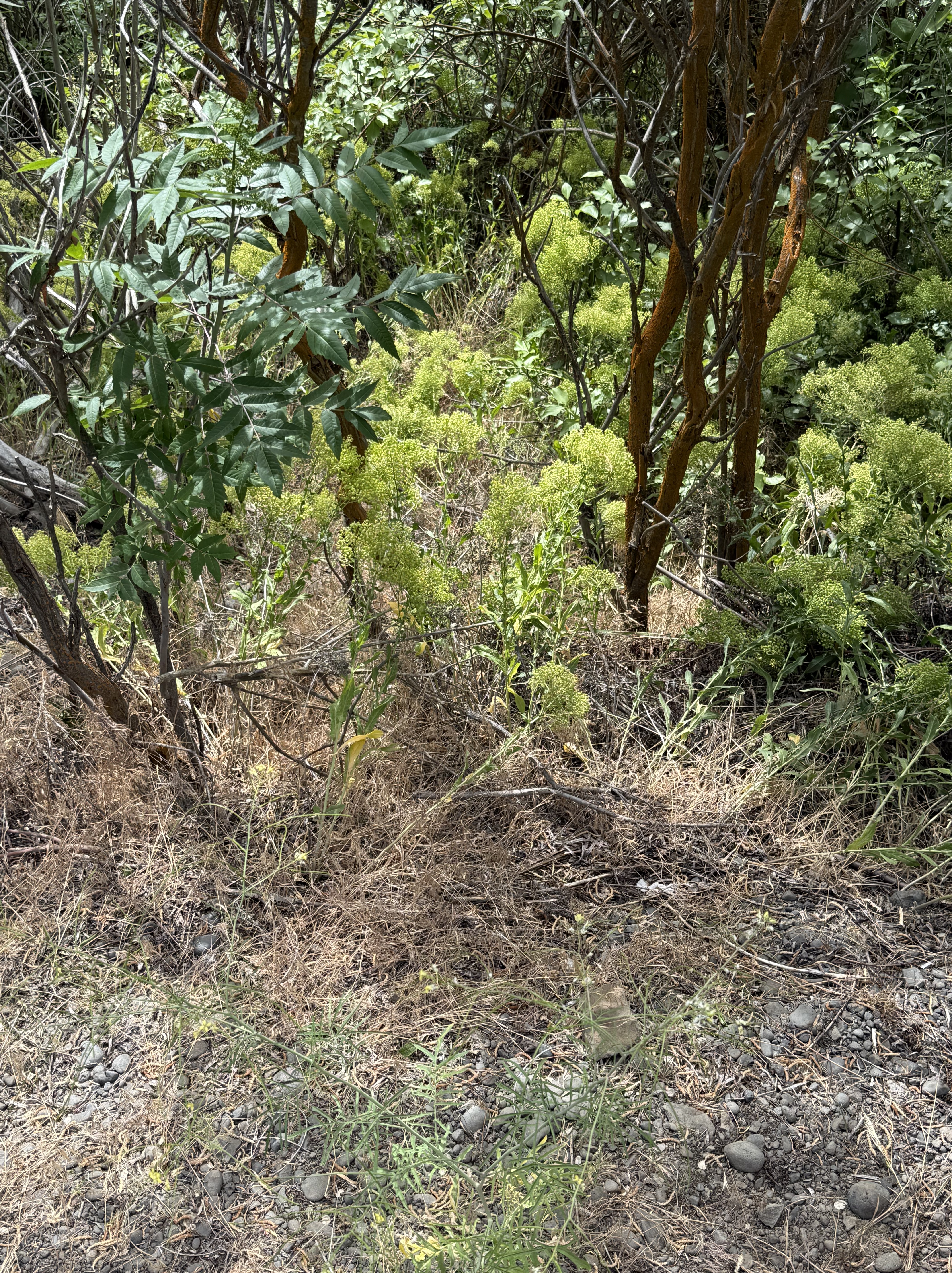
The leafy shrub with dark leaves is snowberry–Symphoricarpos albus (or possibly S. oreophilus, which also occurs around Yakima).
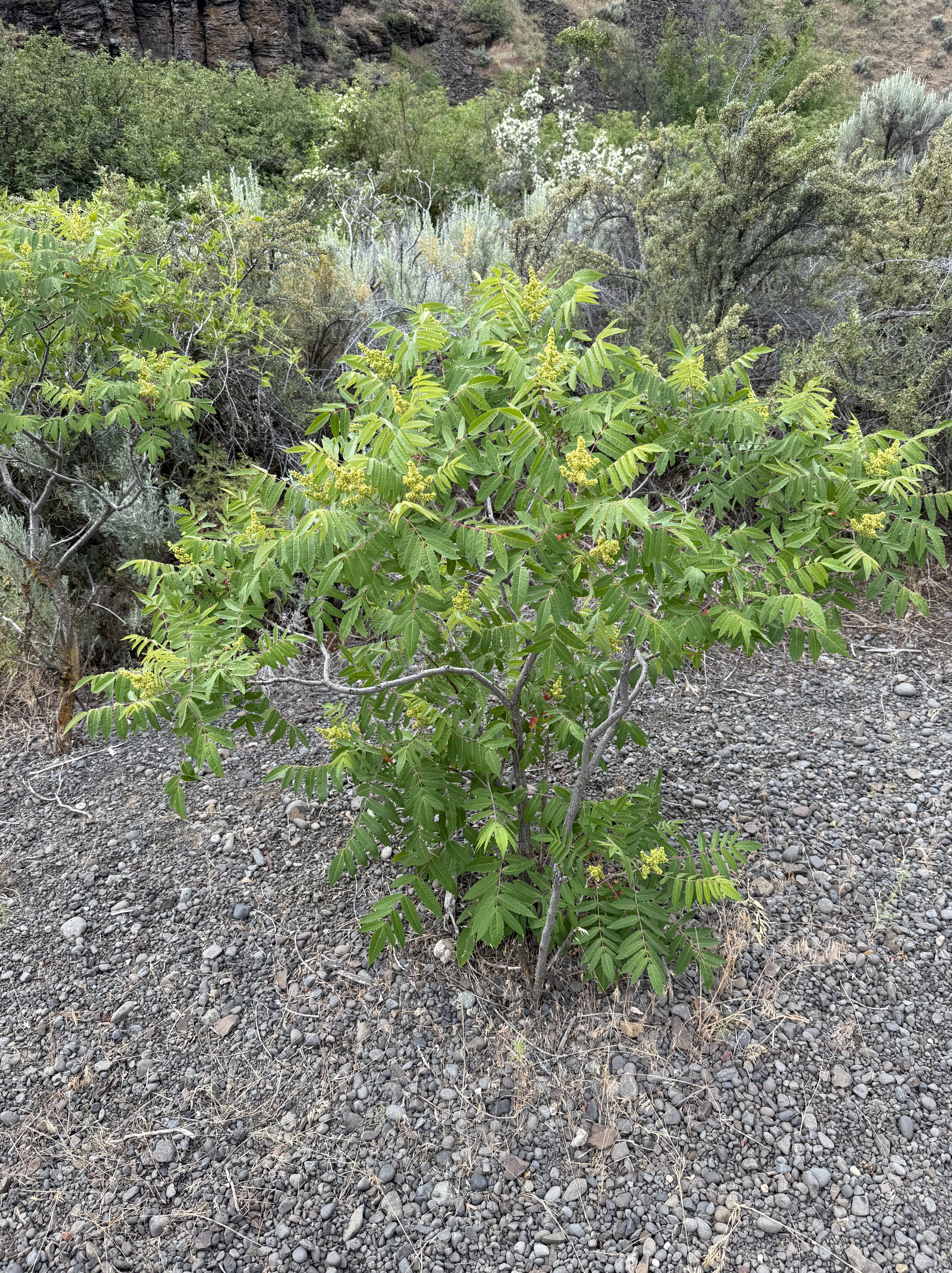
The low, brightly colored shrub with straight stalks is probably wax currant (Ribes cereum). The bright green is small leaves and the small patches of pink–barely visible in the photo–are the flowers. These are both native plants.
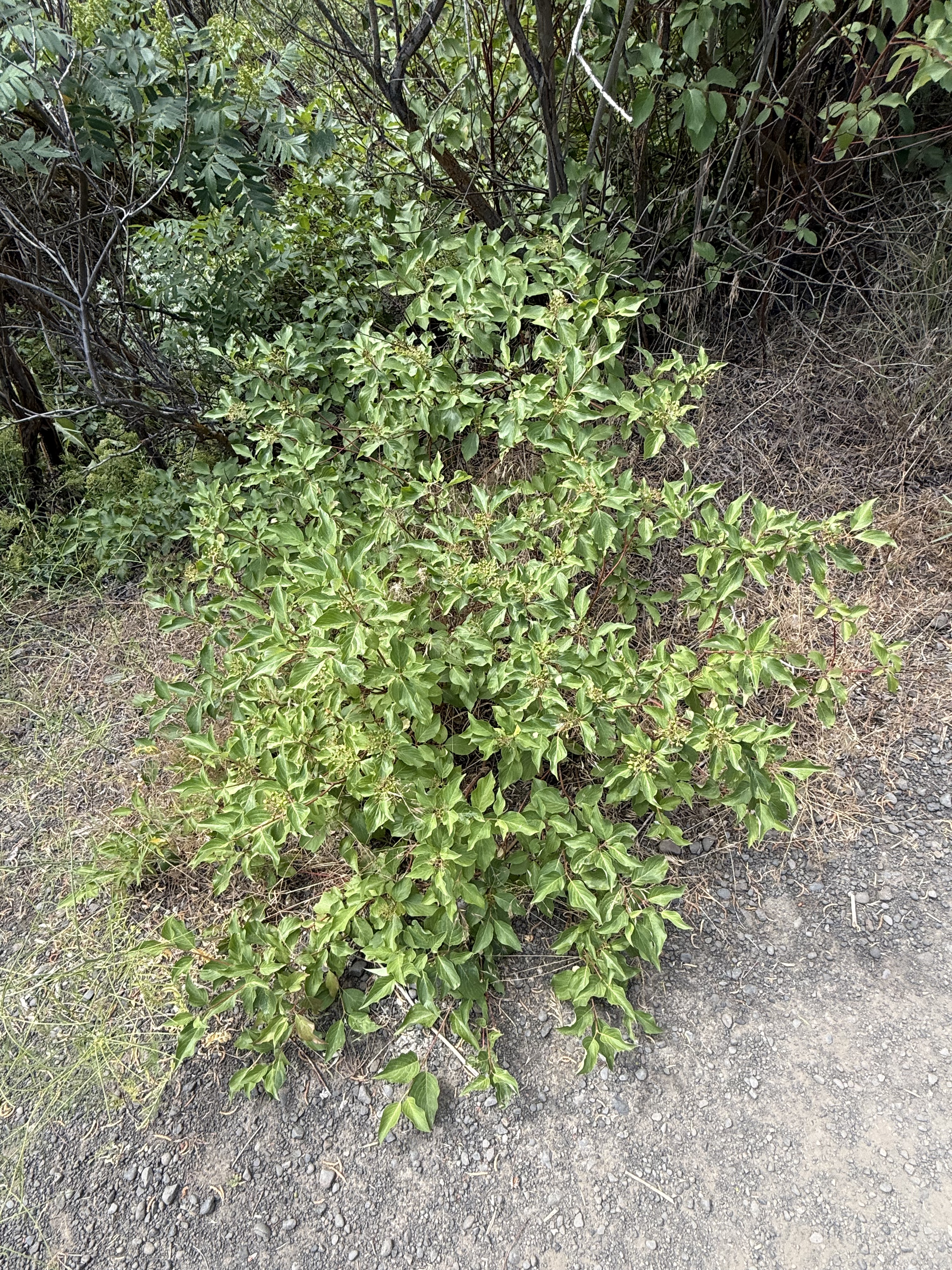
CoPilot wasn’t so sure about this, but it might be Creek or Red-osier Dogwood (Cornus sericea). This specimen was growing in the bottom of the canyon, not far from Cowiche Creek, which is a natural location for this native riparian species. It will probably become a small tree.
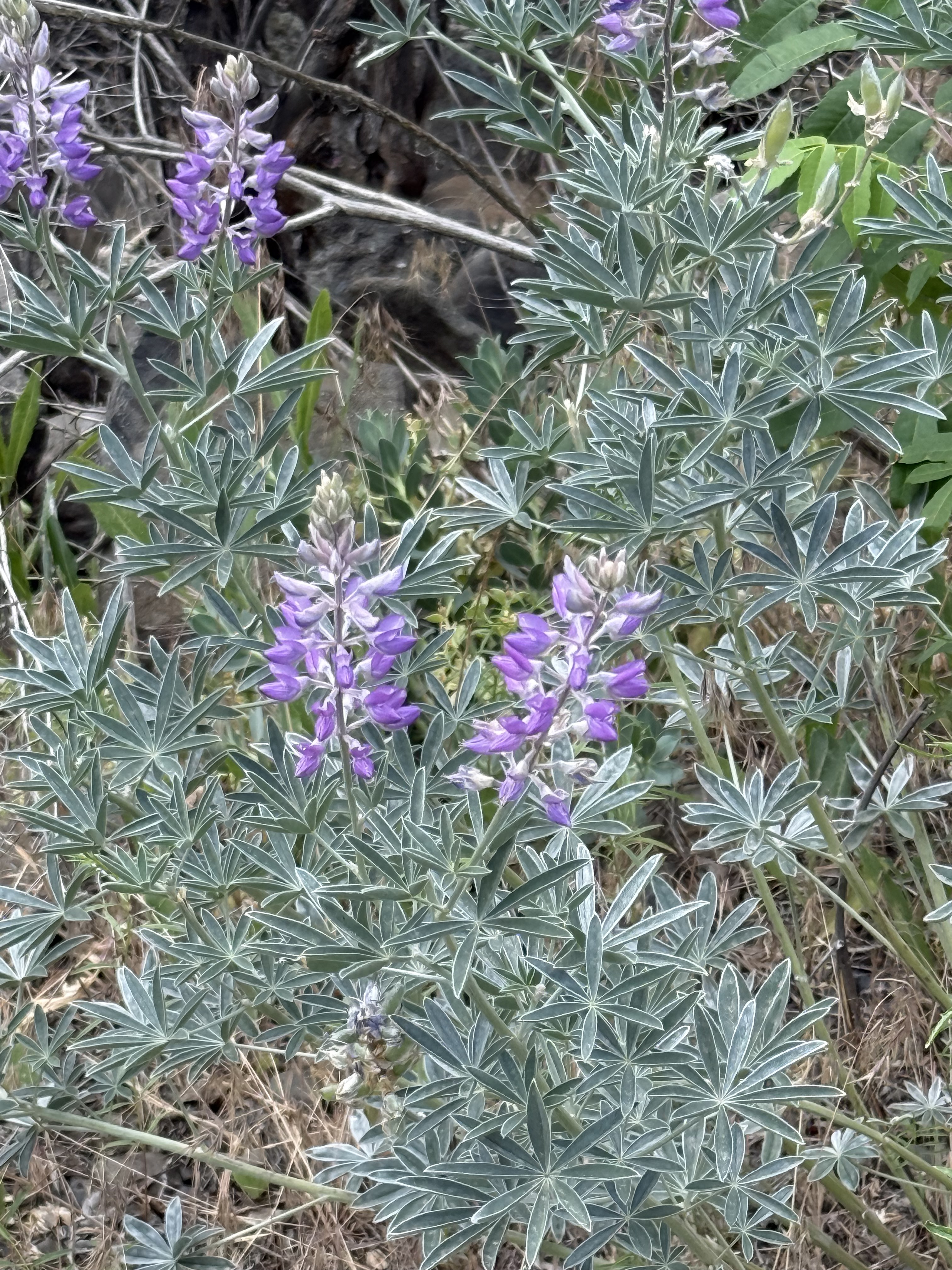
This is my favorite from the walk. Silky lupine (Lupinus sericeus) is one of the signature wildflowers of eastern Washington. I sure am glad we caught them in bloom.
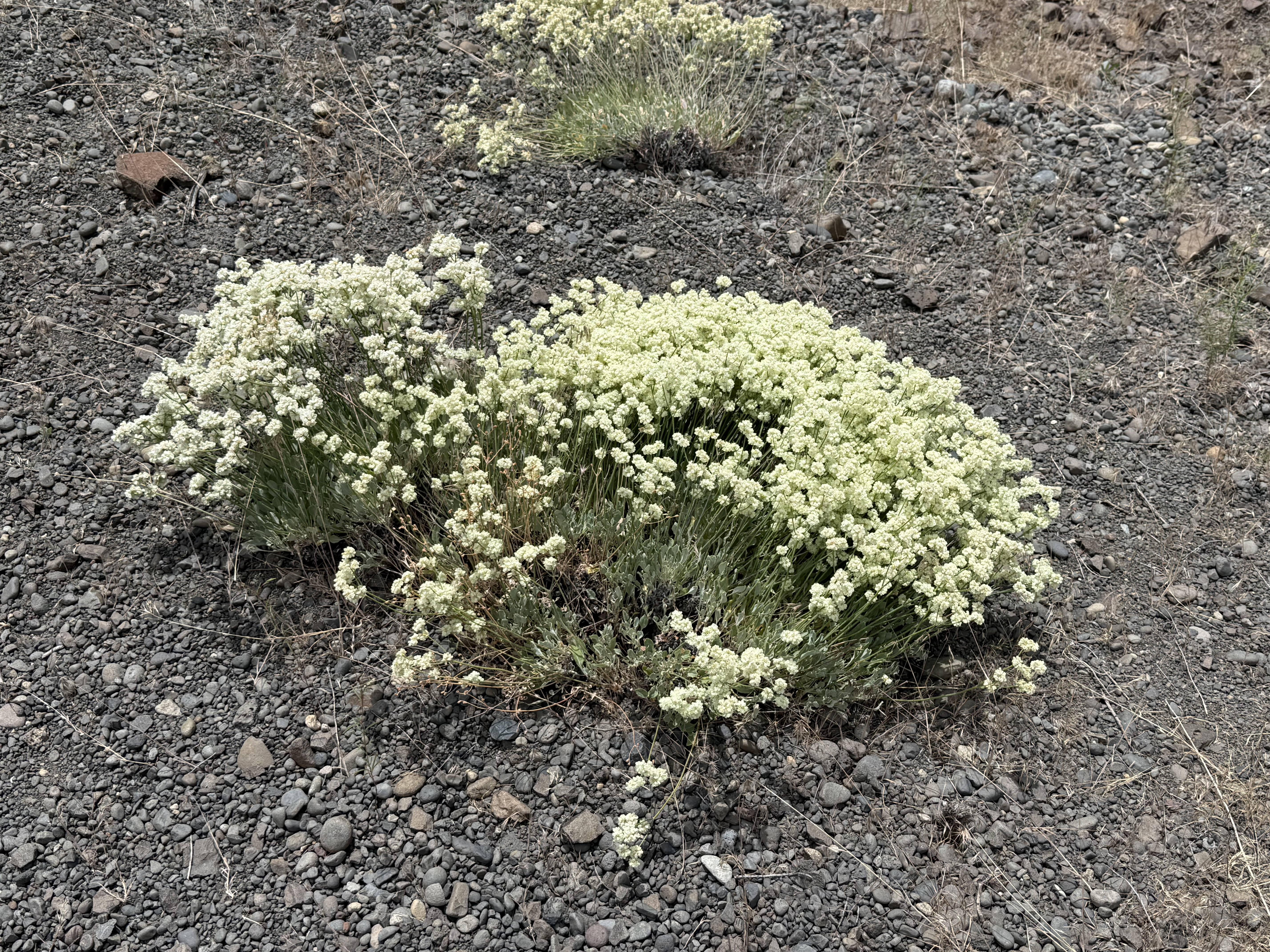
This looks like Pale‑stem buckwheat (Eriogonum heracleoides), another native wildflower to the shrub-steppe habitat.
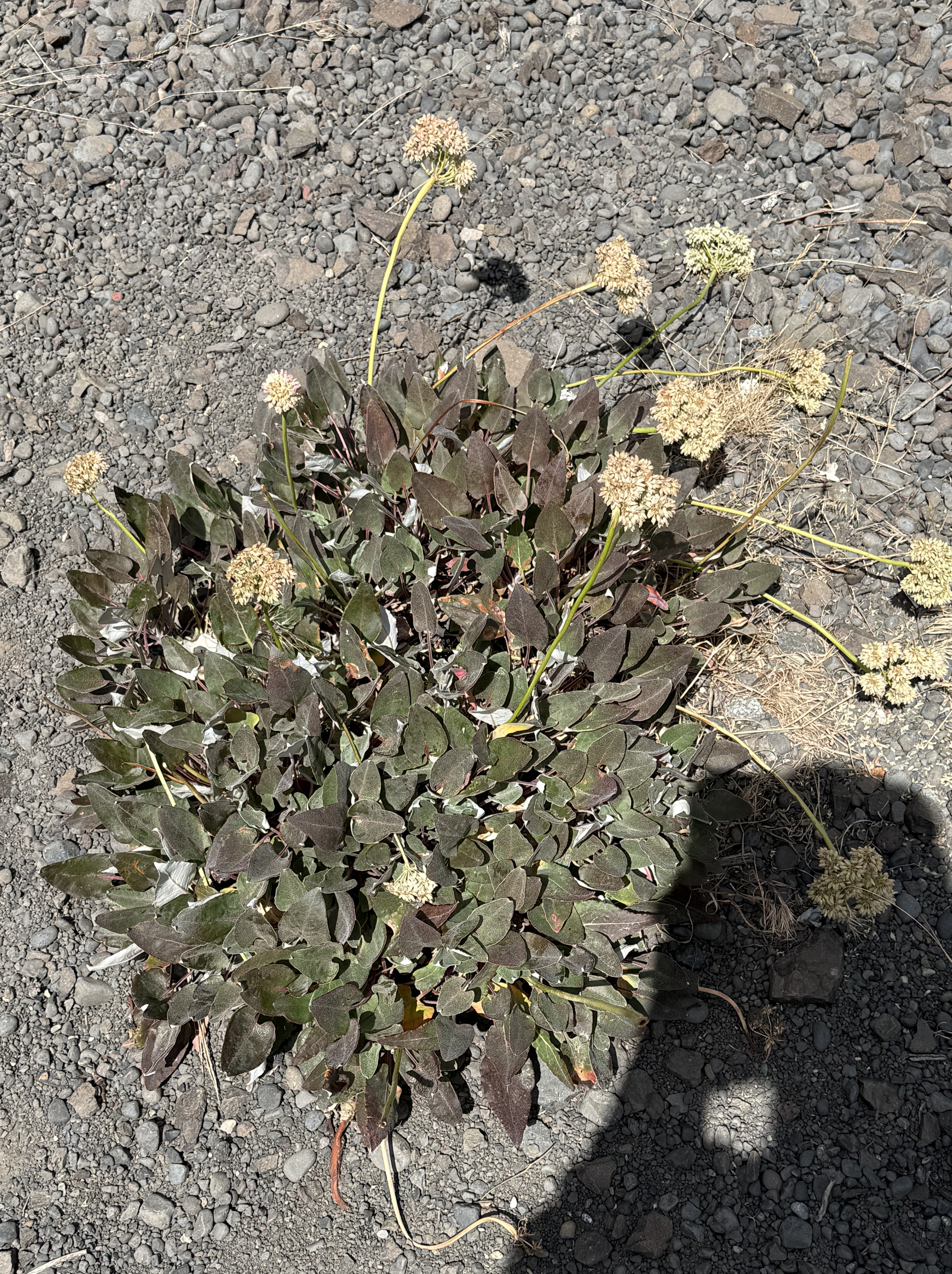
My untrained eye thought this was Pale-stem buckwheat, but CoPilot pointed out the different leaf pattern and color. This is (probably) Sulphur Buckwheat (Eriogonum umbellatum), another common wildflower to Yakima County’s uplands.
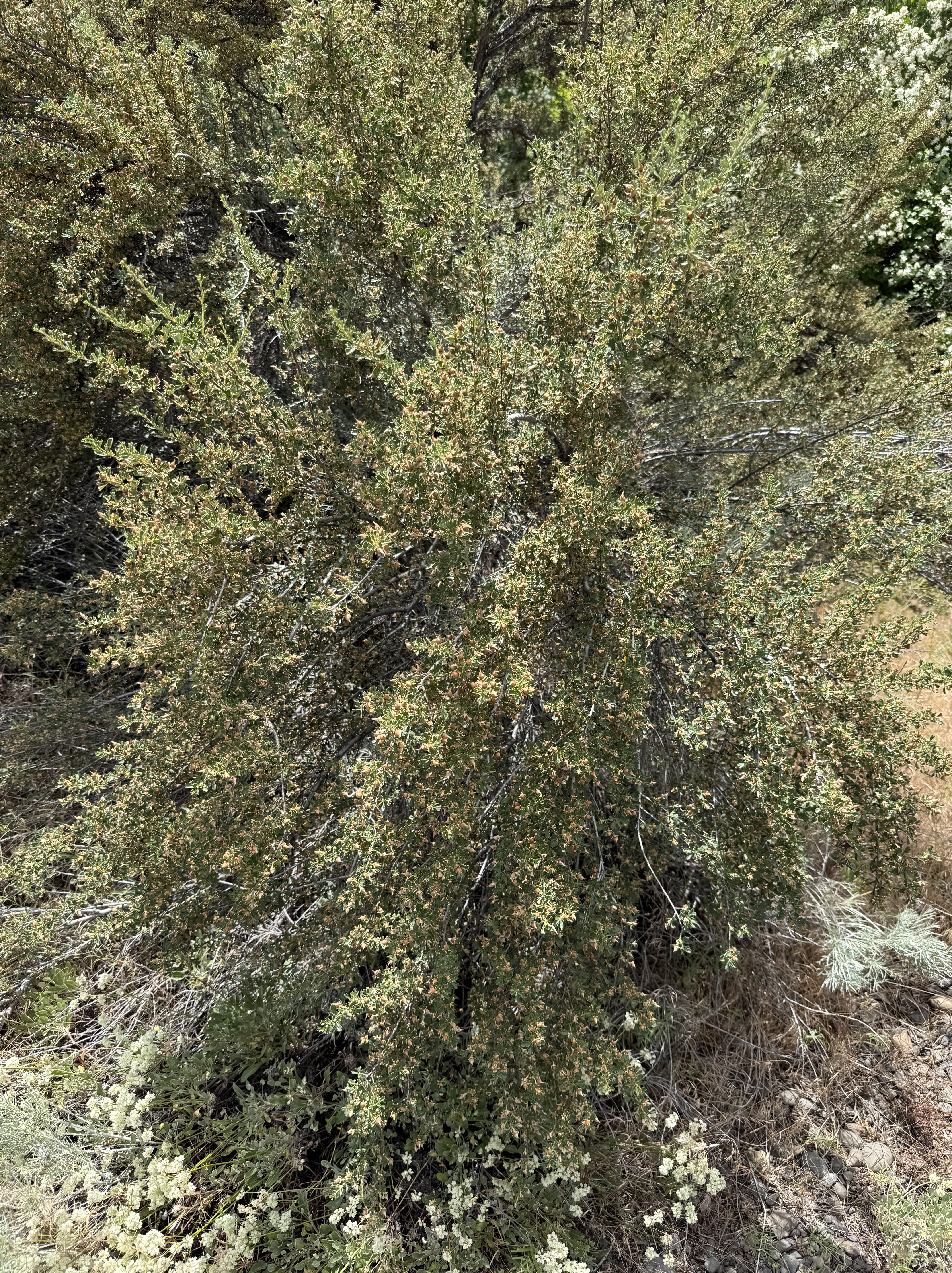
Antelope bitterbrush (Purshia tridentata) is a foundation species of the steppe. This young one had lots of flowers, but the old ones have bare branches; and groups of them grow and die together in cohorts after a disturbance like a wildfire. Yet another native plant.
After some discussion, and sharing a close-up, CoPilot swears (hahaha) this is Woods’ rose (Rosa woodsii). However, its justification fits what I see with my own, somewhat confused eyes.
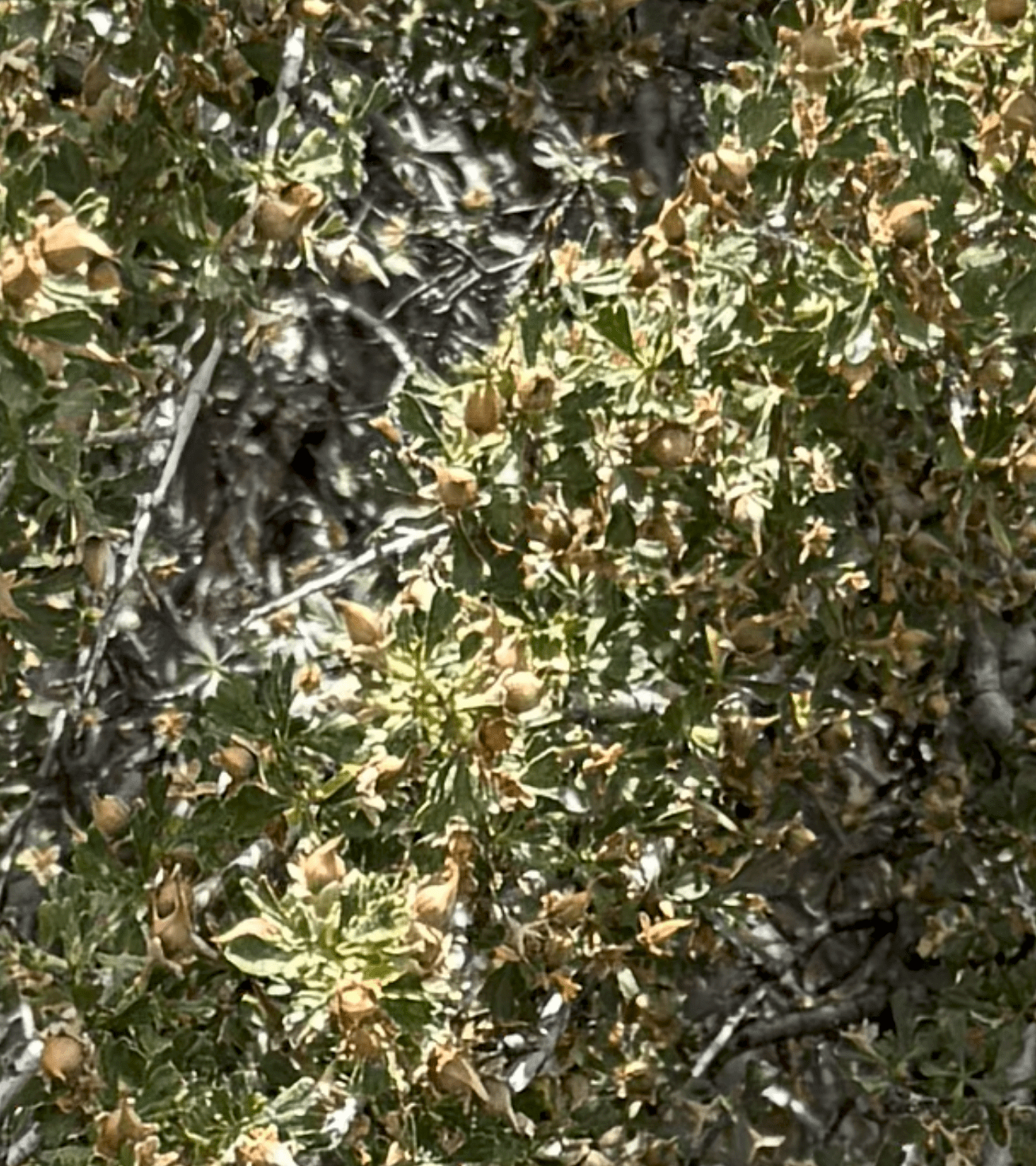
Here’s a close-up of the fruit. The shrub is covered with small nuts that have a distinctive shape, and are definitive for a wild rose. This is another native species to the steppe habitat of Eastern Washington.
This photo, looking across Cowiche Creek, puts it all together for me. On the other side of the canyon we see columnar jointed basalt, several plant species similar to snowberry, bitterbrush, and buckwheat. Along the creek are dogwood and wild rose; and in the foreground is (maybe) big sagebrush (Artemisia tridentata).
When I took this picture, all I saw was a bunch of plants. After carefully examining them with CoPilot, it has become a mixed riparian-shrub-steppe habitat. However, I didn’t see/hear any birds or other animals, even though it was a cool day with temperatures in the mid-sixties.
CoPilot was a great help, but it is not infallible–more like working with someone who has studied some biology/ecology. After all, it is only a Large Language Model, not an AI system trained on recognizing plant species. Nevertheless, it was a great collaborator and I learned a lot from our collaboration.
Ecosystem Notes from Quinault Rainforest
Introduction
I’ve spent the past few months wandering the Olympic Peninsula with my attention fixed mostly on rocks—tilted beds, breccias, sea stacks, and the stories they tell about deep time. But along the way I’ve been noticing the living world with the same quiet fascination. I’m not a biologist and I don’t pretend to be; I can’t name any of the plants I pass. What I can see is how each organism plays a role in the larger system, the way geology shapes life and life responds in turn. These are simply notes from a wanderer paying closer attention.
I’ll try to remember to label these environmental posts as NOTES to avoid any confusion, especially on my part. This first post arises from a short walk on a semi-muddy trail through the Quinault Rainforest, on the Olympic Peninsula. I won’t have much to say about the photos, and all identification will come from CoPilot (aka ChatGPT). I’m certain its identifications will be better than mine after hours of searching the internet.
Quinault Rainforest in Olympic National Park
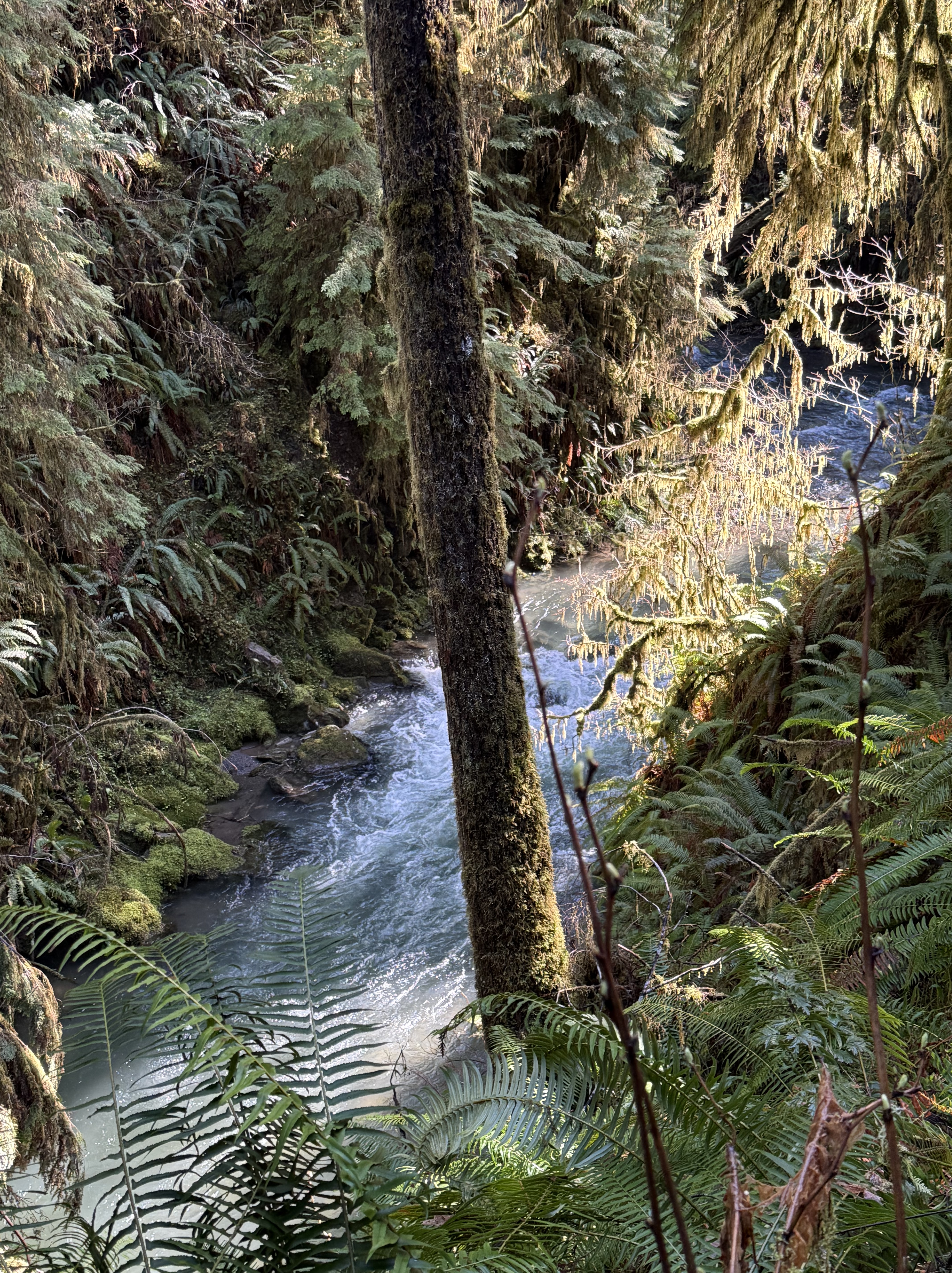
Plate 1. That raging stream about 50 feet below me is one of hundreds draining this temperate rainforest, which gets about 12 feet of rain per year. Note the ferns, which are everywhere, even in the temperate forests of northern Virginia. Ferns must be the most common plant in cooler forests. I am in a narrow strand of Olympic National Park that has never been logged. This is primordial nature, viewed by a geologist, but I’ll do my best.
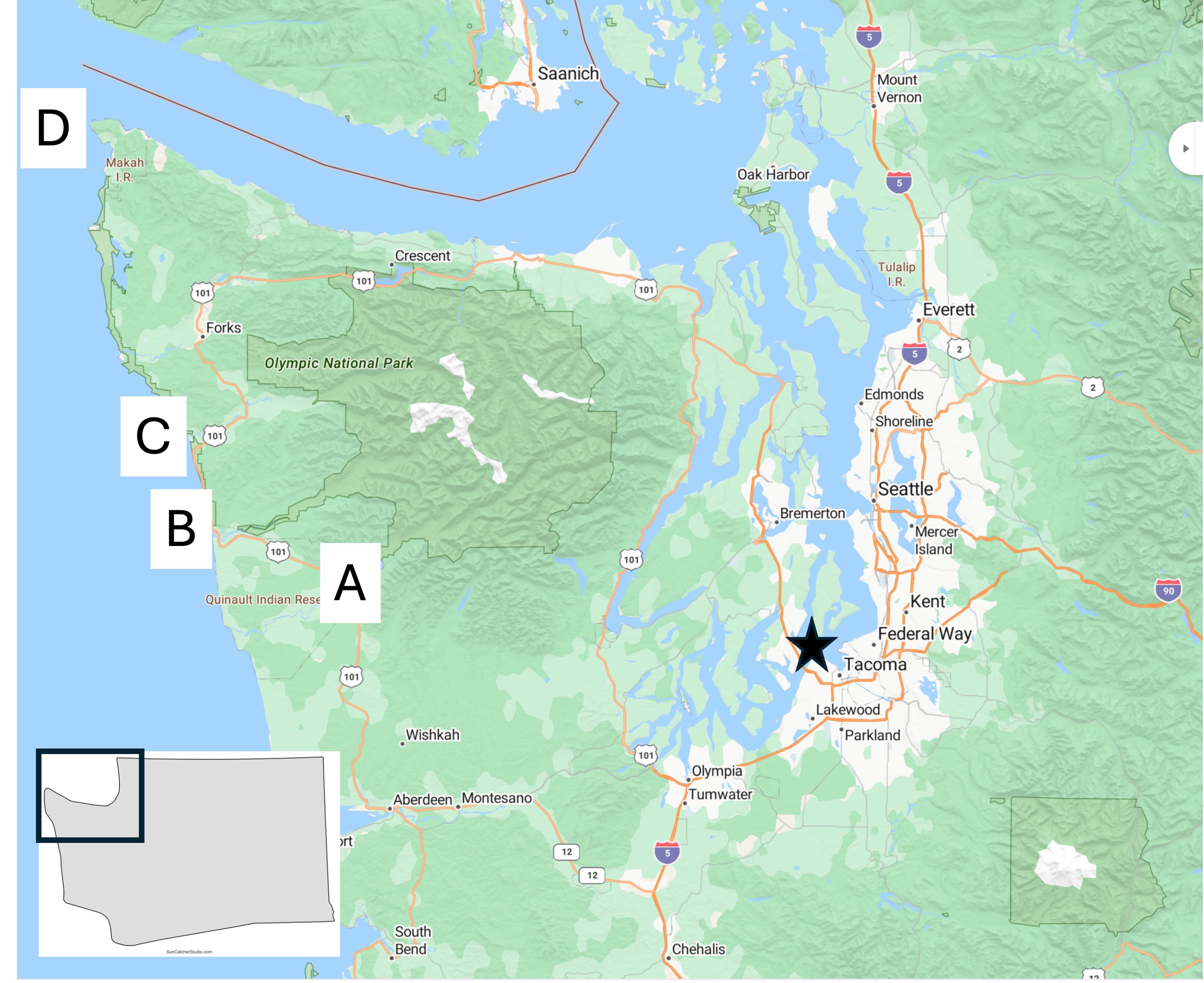
Plate 2. Map of the Olympic Peninsula showing the areas I reported on in previous posts. I’m going to be focusing on Site A today, with a few photos from D.
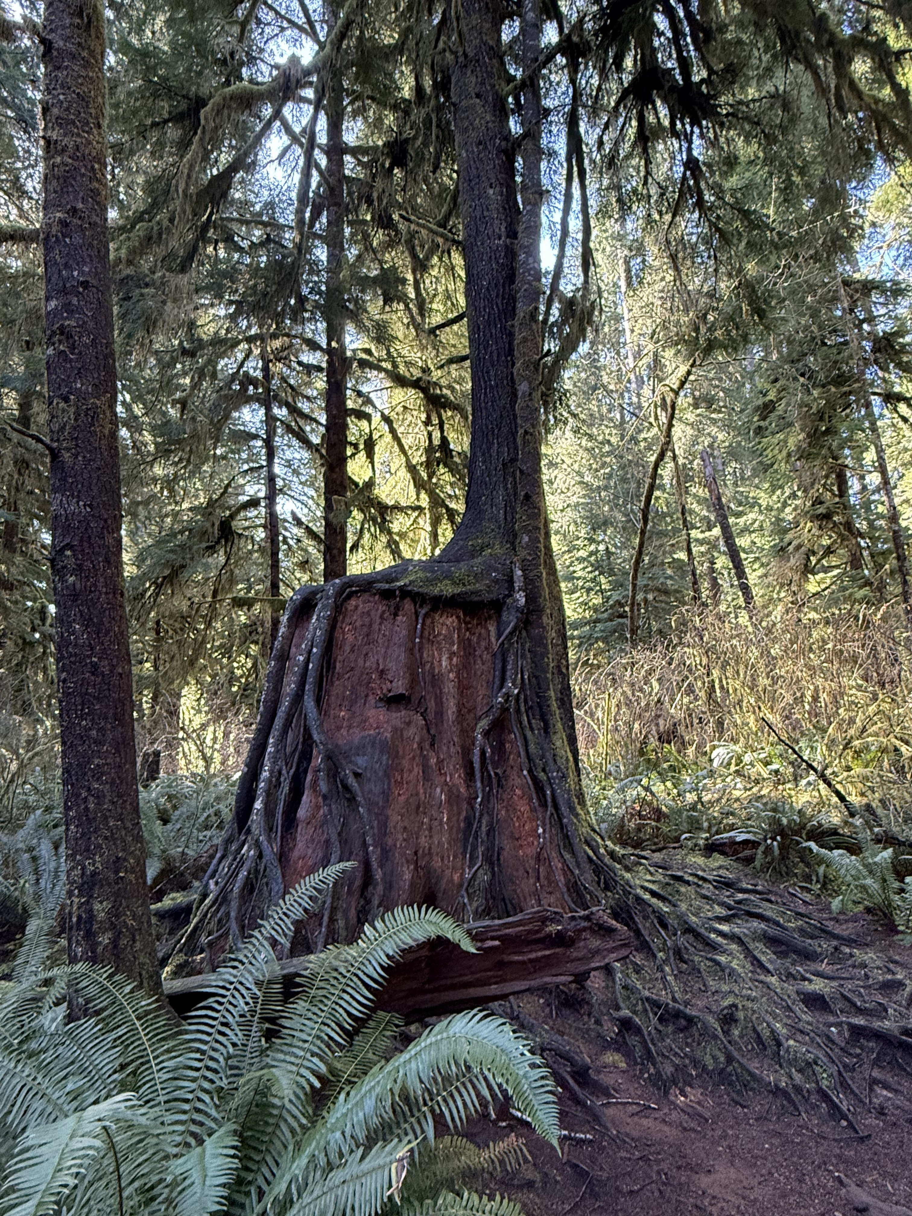
Plate 3. I haven’t seen this anywhere else I’ve lived, not even northern Virginia, but they occur everywhere here in Washington. Apparently this is a common occurrence in rainforests, where the ground is a dangerous place for seeds. I couldn’t identify the species in this photo, but this practice is very common for hemlock.
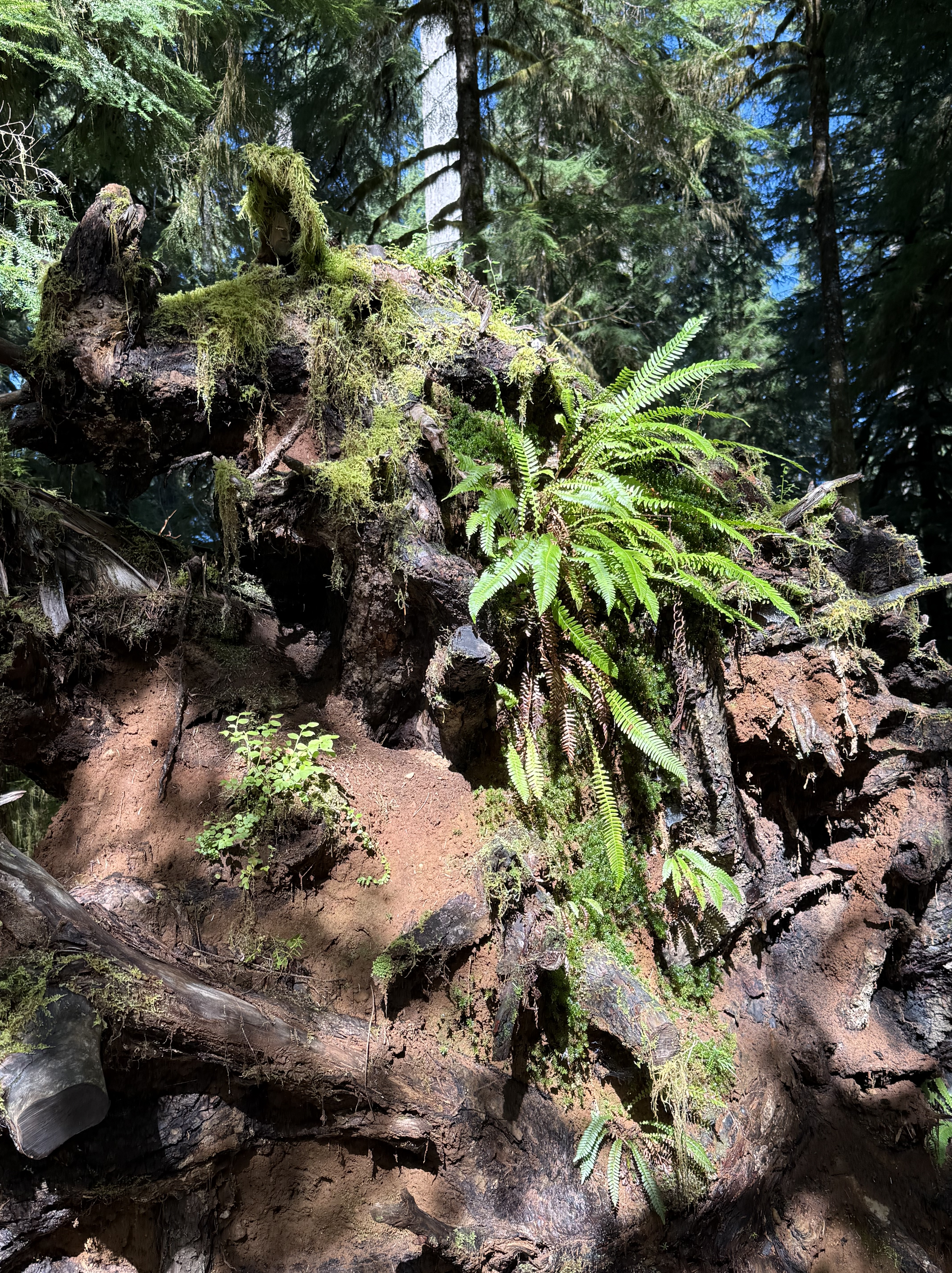
Plate 4. This pile of debris is a large log turning into compost and supplying nutrients to a variety of plants. The top of the photo shows the base of a young tree growing out of all this chaos. According to CoPilot and the Olympic National Park map, this area has never been logged, so I am in wonder of this pile of “forest garbage”. Is that sandy soil I see? Where did it come from? I don’t know.
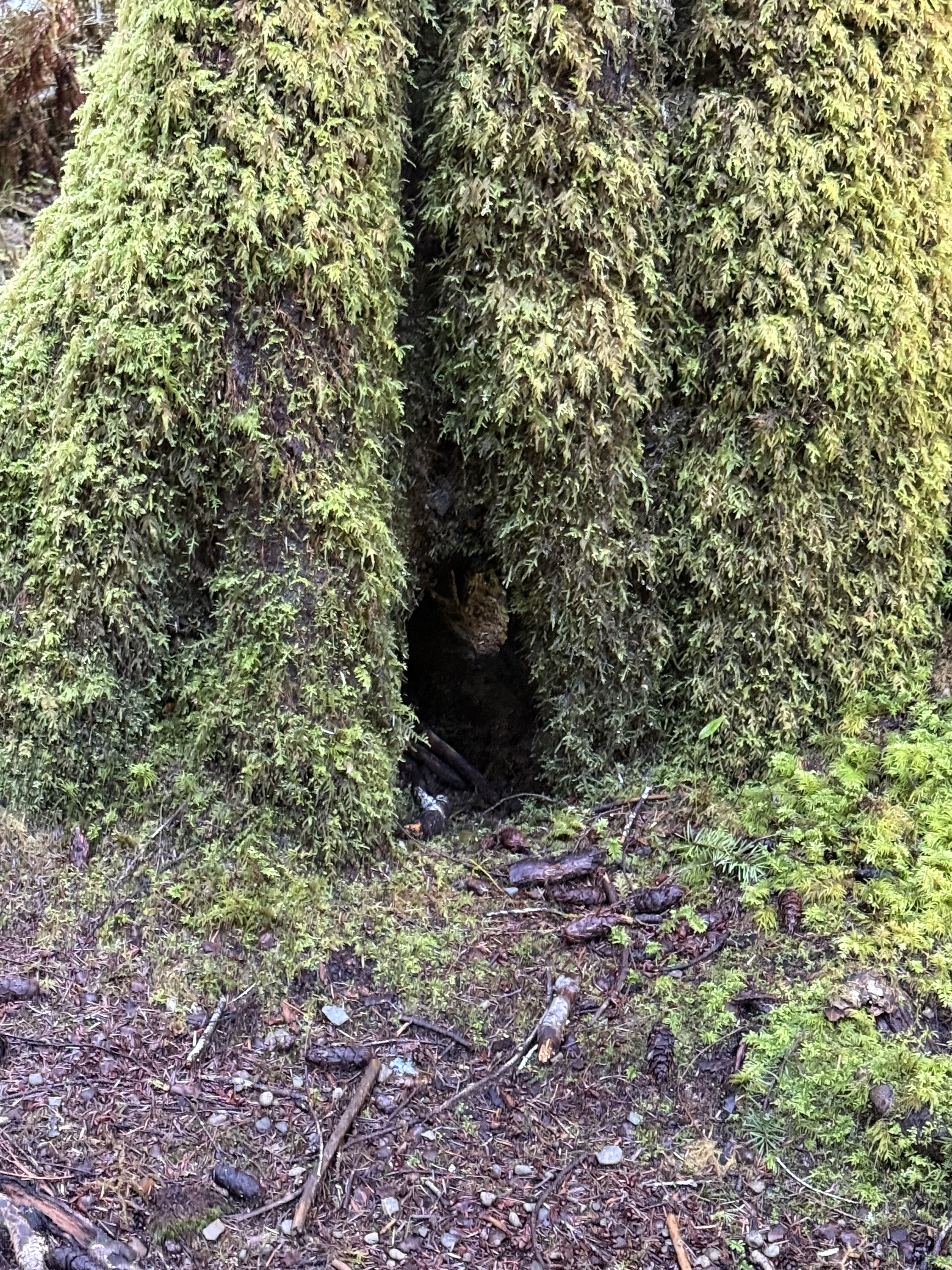
Plate 5. If you look close in the exact center of this photo, you’ll see daylight on the other side of the base of this unidentified tree. It’s about six-feet in diameter and covered with an epiphyte community of mosses and liverworts. Those aren’t leaves or fronds, but communities that mimic ferns–for their own reasons.
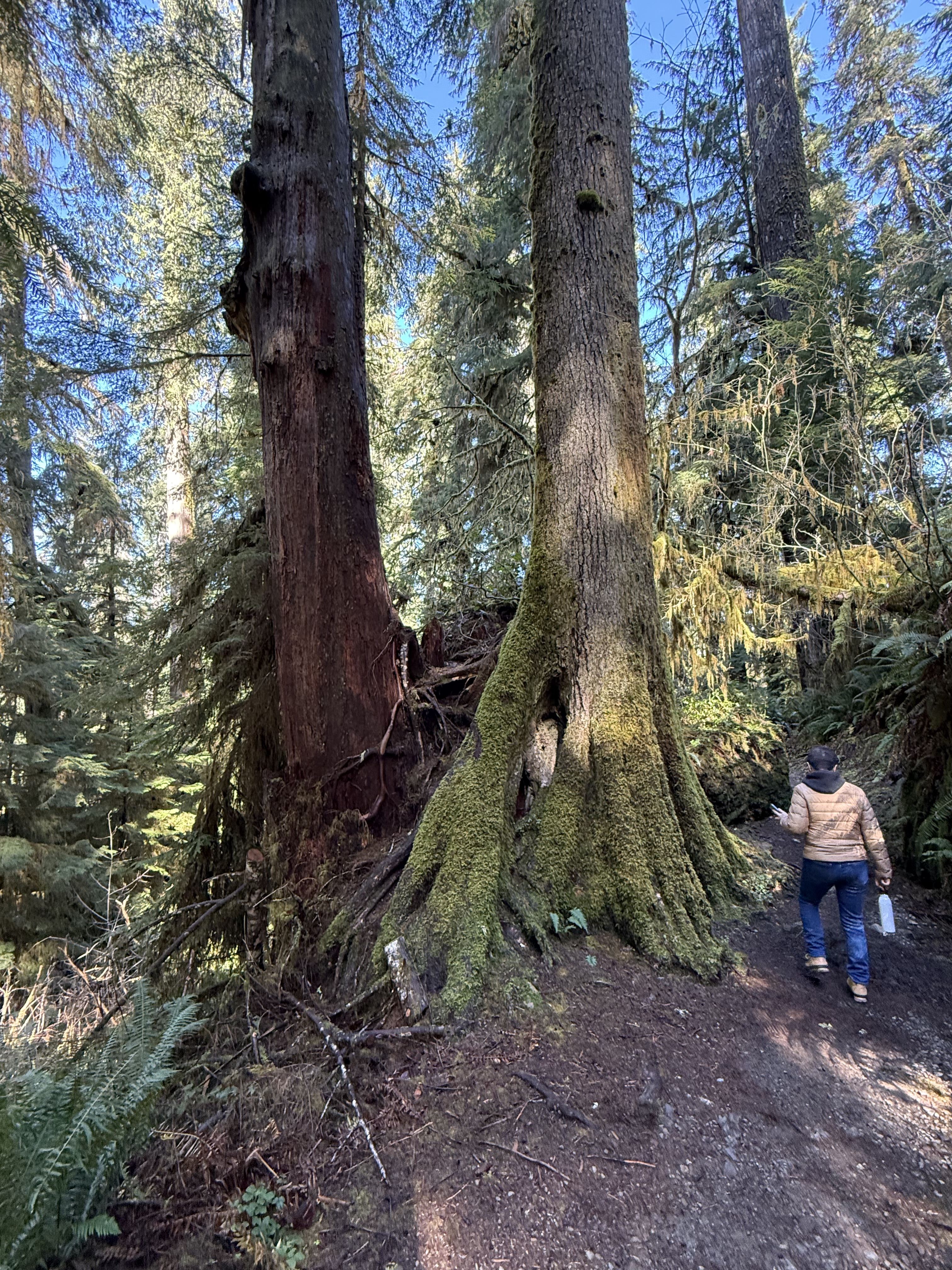
Plate 6. Here’s an example of a Western Red Cedar that has grown into a mature tree after being nursed by a stump. I guess it will eventually absorb the rotting stump and grow to full height, but this is the largest I’ve seen so far in the region.
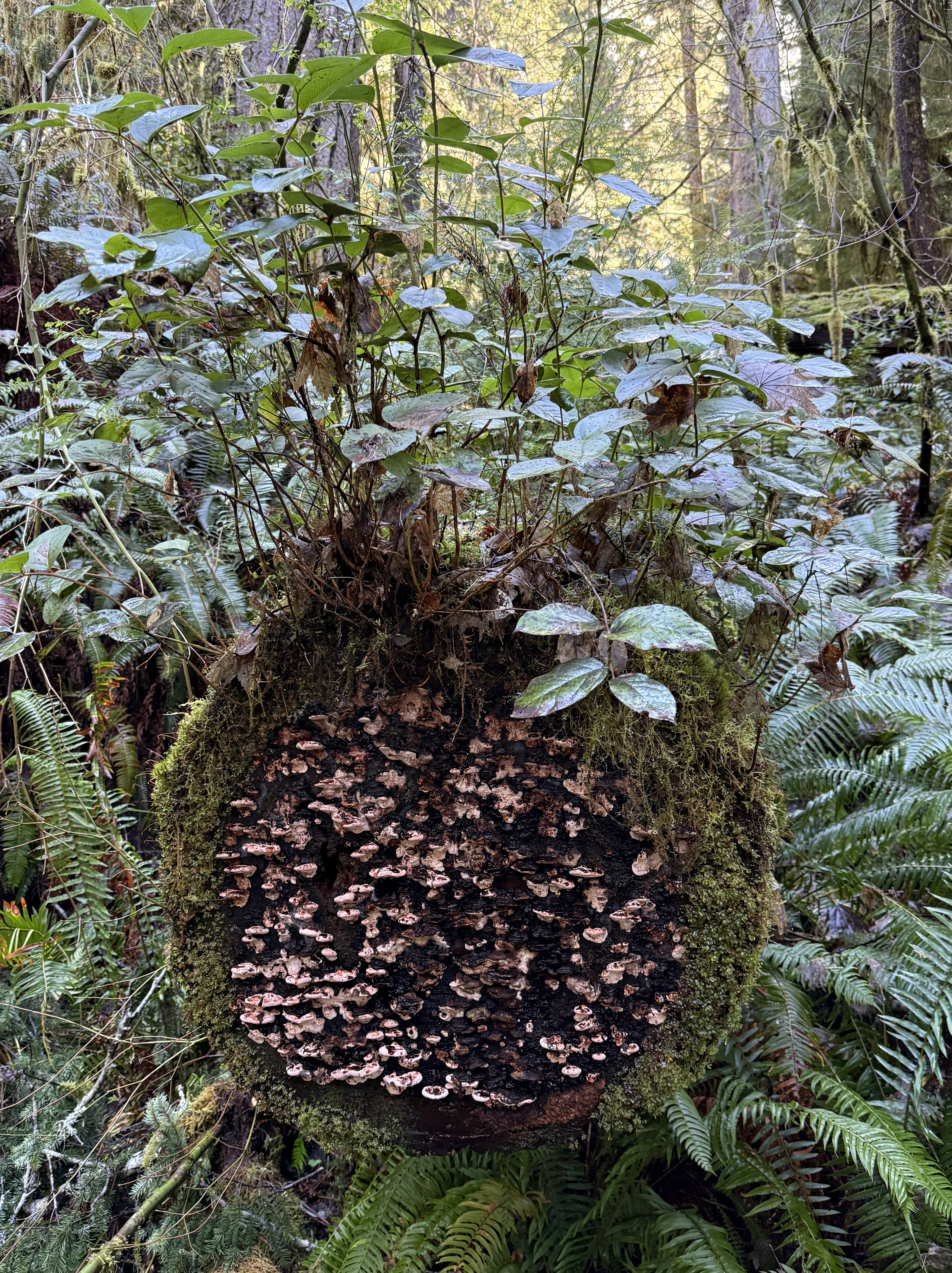
Plate 6. This miniature ecosystem caught my eye, but I had to turn to CoPilot to get an idea of what’s going on. As a tree trunk decays it goes through five stages: 1) moss; 2) liverworts; 3) fungi; 4) shrubs; and 5) young trees. This one seems to be in stages 1-4. I didn’t see any seedlings on it. The shrub is probably huckleberry and the mushrooms a bracket fungus, probably Trametes or Stereum.
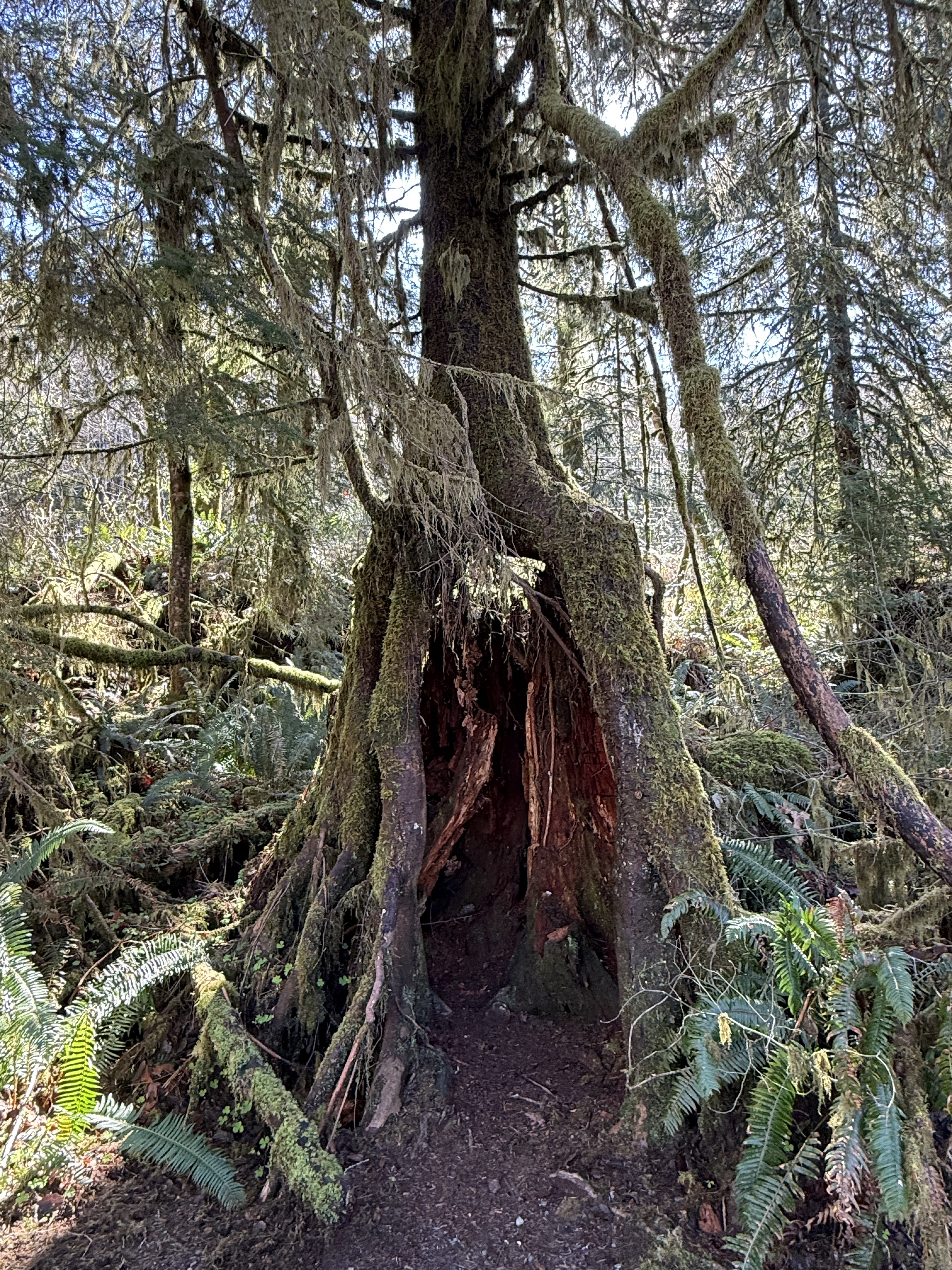
Plate 7. I am fascinated by these nurse trees after seeing species of fig trees in Australia that devour living trees, like a giant fungus or alien. These are nursing on dead trees, however, so it isn’t as gross; but this one is now standing on its own legs after the original stump has begun to collapse.
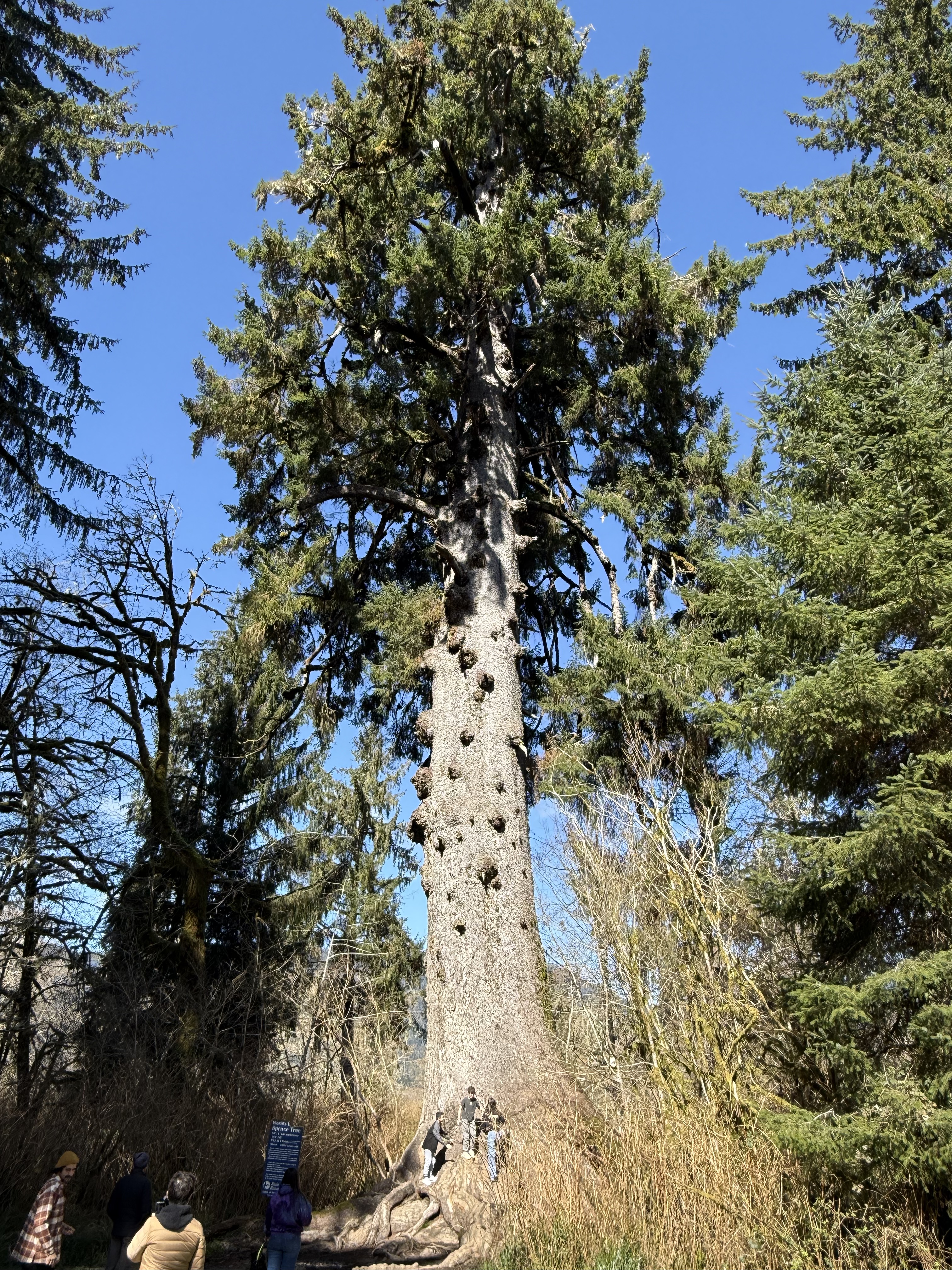
Plate 8. This is the largest Spruce tree in the world. It’s 191 feet tall and about 1000 years old. It is growing in a swampy wet land at the inflowing stream to a glacial lake, Lake Quinault.
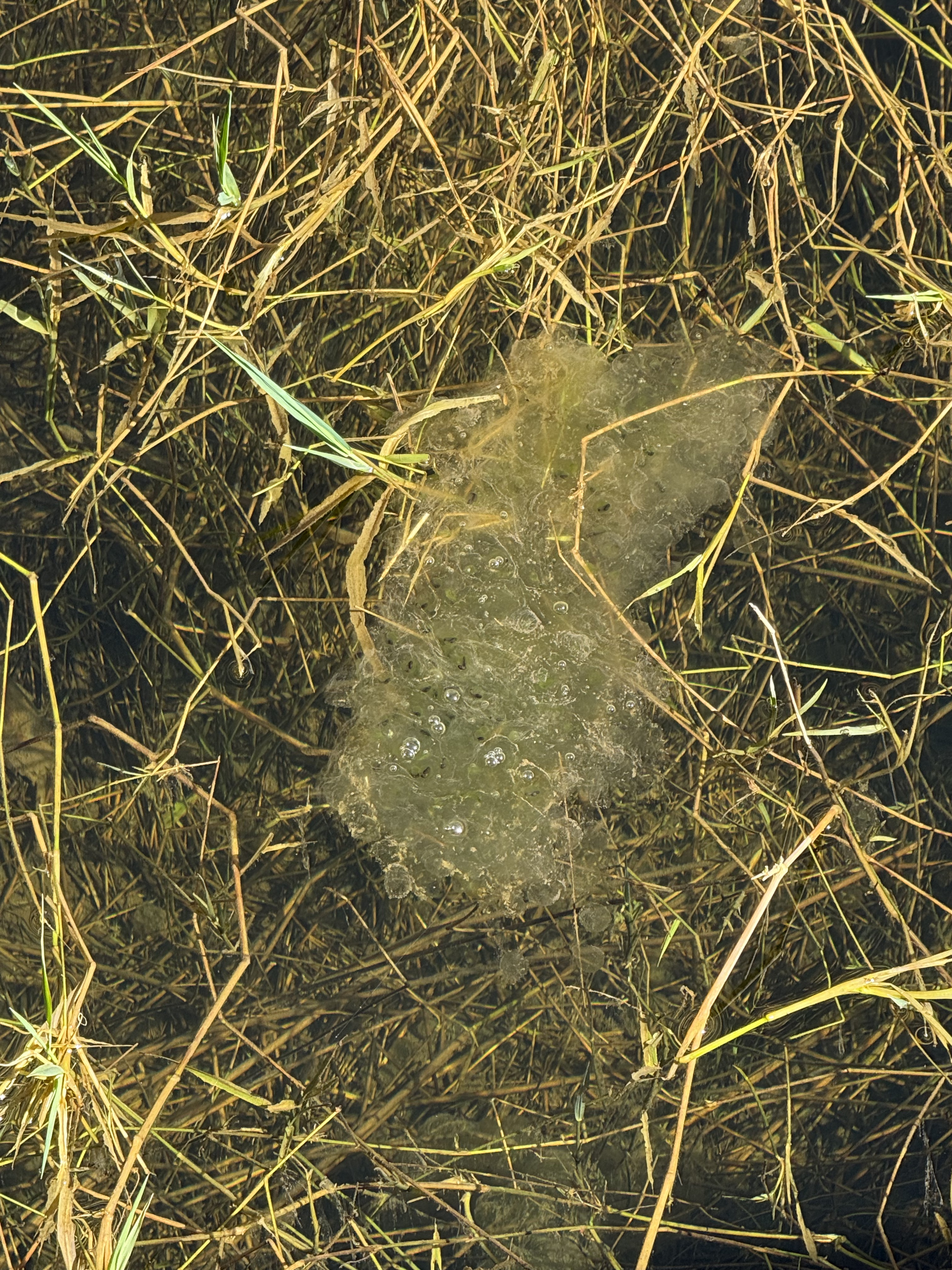
Plate 9. I thought this was toxic waste until CoPilot took a look at the photo: this is a mass of frog eggs (probably northern red-legged frog). There were several more at the shallow, marshy wetland where a stream fed Lake Quinault. The water is so clear you can see the bottom, which is only a couple of feet down.
Kalaloch Beach in Olympic National Park
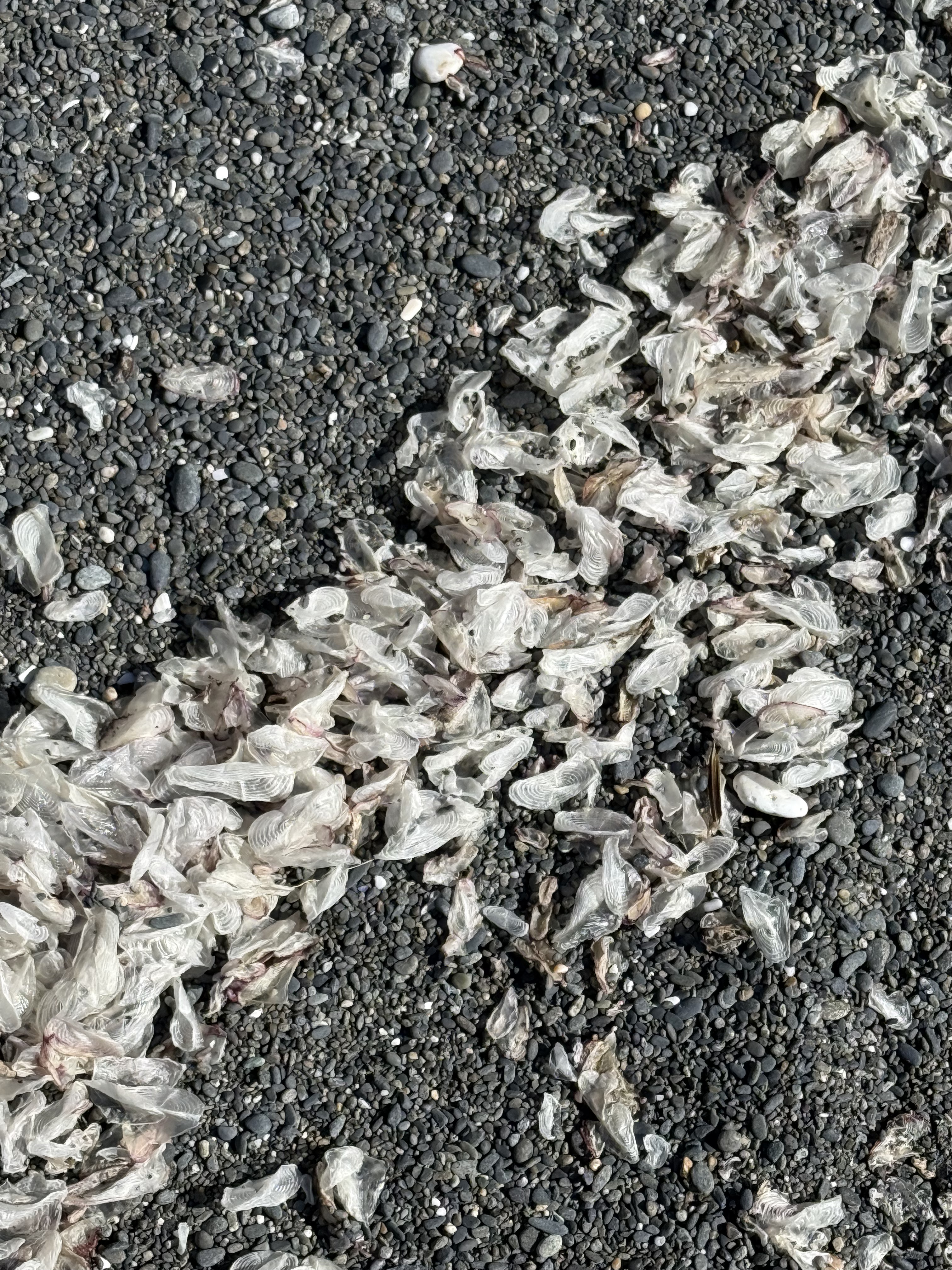
Plate 10. This one was a doozy. These objects are one-two inches long, thin, translucent, and oval in general shape. At first, CoPilot suggested insect wings (until I told it the size), then gull secondary feathers (until I said, “no way”), then settled on small fish cranial bones–e.g. the opercula, the bone that covers the gill. I asked for references, but it supplied me with titles and no links (how did it find them?). I spent longer on this photo than I wanted to. I don’t fault CoPilot for its ambiguous response because I found nothing when I looked very specifically. This phenomenon is either so common that no one bothers mentioning it, or infrequently observed that no serious beachcombers have stumbled across it. I’m going to have to agree (for now) with CoPilot that these are small bones from a school of fish that was decimated by either predation, coastal fishing, or disease and only these translucent cranial bones survived by floating, until waves concentrated them on this beach. This is the only beach where I saw them. I guess there are no easy answers to some questions–unless someone who reads this is a marine biologist.
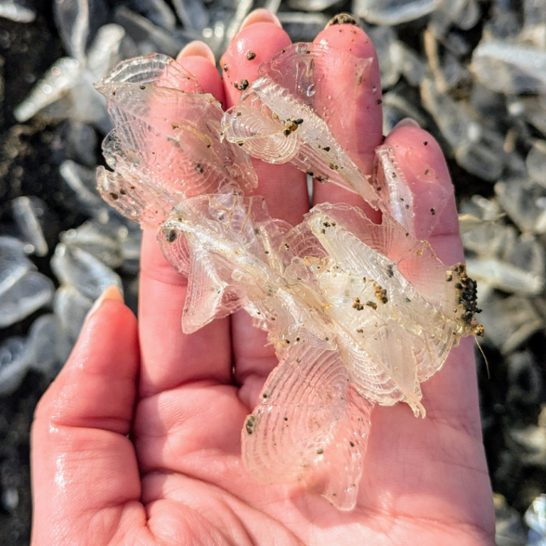
Plate 11. I solved the mystery of the white objects on the beach (Plate 10). I spoke to an ecologist I know who suggested they are a Hydrozoa called Velella-velella, which floats on the ocean like a jellyfish. They are a colonial organism that is blown about by the wind. They don’t swim so they are easily blown onto a beach and carried by waves. (Here’s a good article about them.)
Cape Flattery
I reported on this amazing location in a previous post. You can scan that post to get an idea of where these photos were taken.
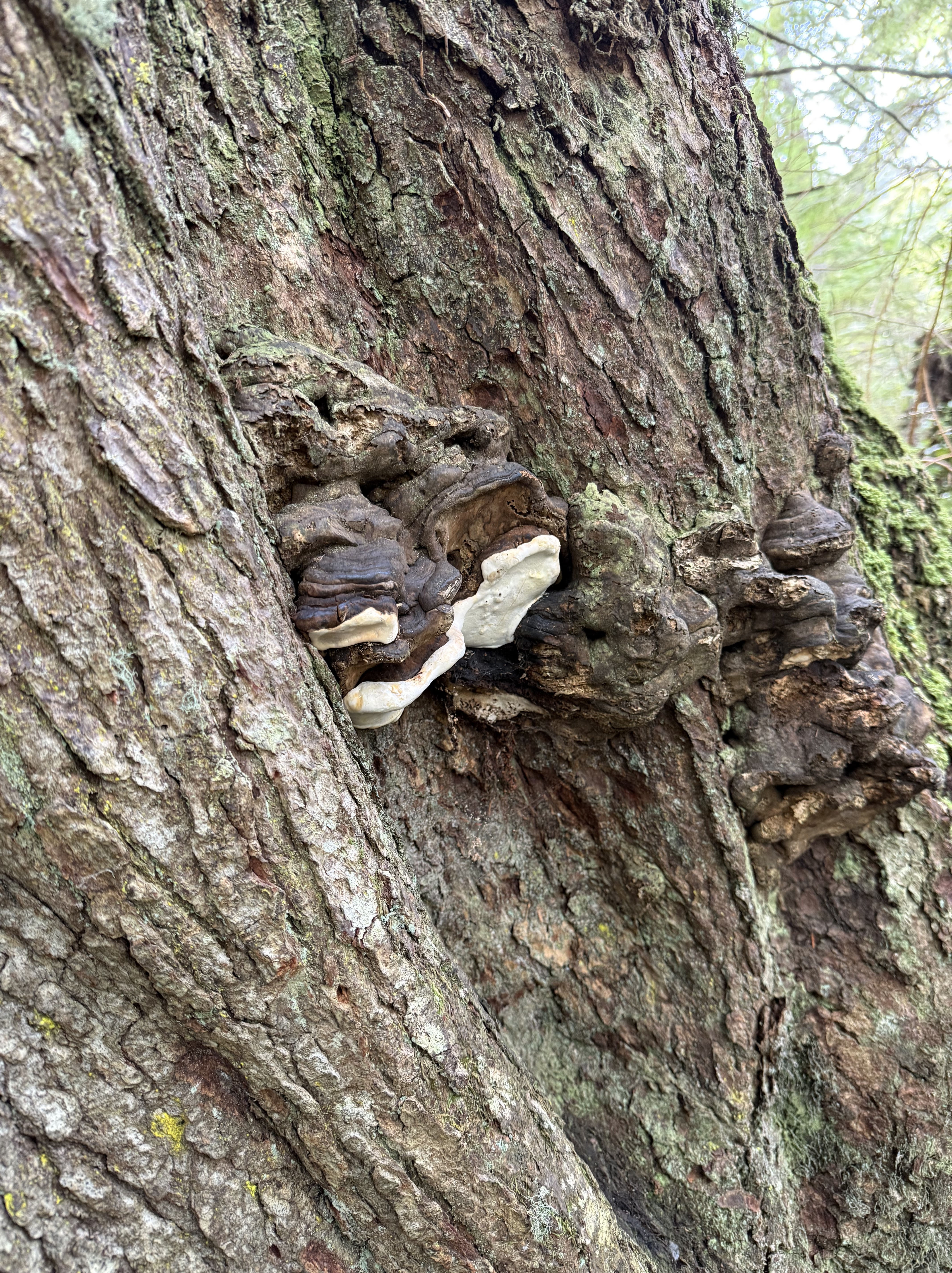
Plate 11. I don’t know if this living (it looked healthy to me) tree was stressed or not, but CoPilot thinks these are perennial bracket fungi, which favor environmentally stressed conifers. There were only a few on this tree. I noticed that this forest didn’t show nearly as many signs of decay as Quinault Rainforest, despite its exposed location.
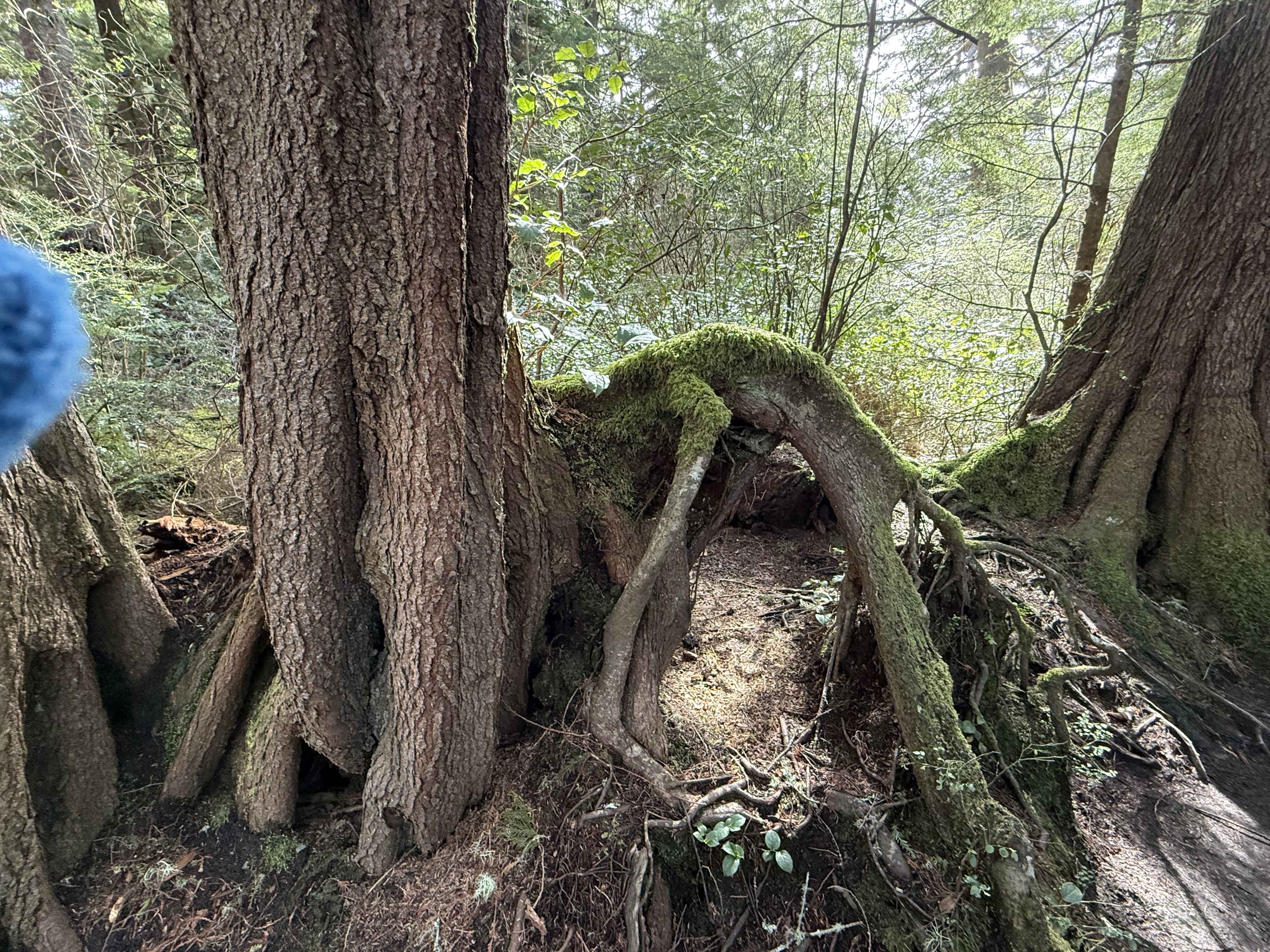
Plate 12. I had to throw this photo in because the root growing out of the tree(s) on the left looks like a dog that got its head caught in a hole, and died there. Its limbs of limp. Overactive imagination, I know. Nevertheless, this is a bizarre image because the dog is lying on top of a mound of soil. I’d bet there was a stump there that has decayed because the trees visible in this image are both composed of multiple trunks. A large tree died here (like the dog) and these are its adopted offspring. I would add that Cape Flatters, which is part of the Makah Reservation, has never been commercially logged. This is old-growth forest and this is a naturally occurring phenomenon.
Summary
Moisture drives everything on the Olympic Peninsula, soaking old volcanic and sedimentary foundations until the forest grows straight out of its own decay. Fallen logs become elevated nurseries, their wood breaking down under fungi and mosses until they’re more sponge than tree. Hemlock, cedar, and huckleberry take root on these platforms, sending roots around stumps and into the thin soils draped over ancient bedrock. Even the beaches tell the same story: waves sorting bones, shells, and driftwood carved from headlands shaped by tectonics and storms. It’s an ecosystem built on slow collapse and constant renewal.
Acknowledgment
I am experimenting with using CoPilot (aka ChatGPT) to help as I pursue my growing interest in ecosystems. I have been up front about where it contributed. It has been a great help, as well as an inspiration; if not for CoPilot, I wouldn’t have had the time of inclination to add these ecosystem NOTES to Rocks and (no) Roads. In fact, I’m tired of this entire series of posts, for which I get no compensation other than sharing my observations of the world. As a final note, CoPilot wrote the Summary and I stand by it.
Now I have to think about more than just rocks…
The Lemay Auto Collection
The museum occupies the entire grounds of a 20th century boys school, so they have a lot of cars!
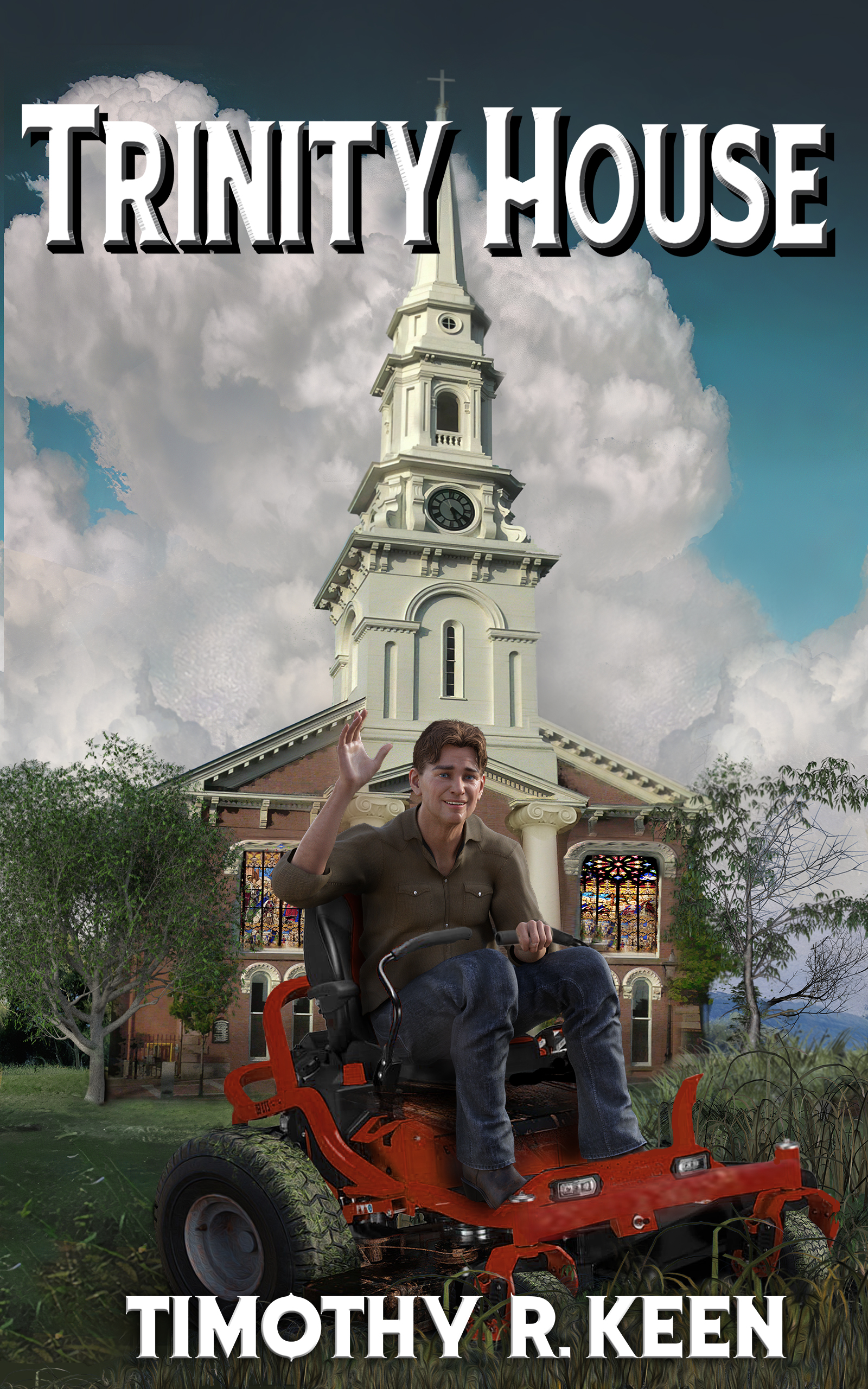
Trinity House
Trinity House was written during the Covid pandemic and thus expresses my frustration with the divisions I was watching grow within American society. I didn’t want to write a dramatic story but that’s probably what it is. As the author I accept full responsibility for this dark comedy that attempts to explore the relationship between superstition and innate human behavior.

The professionally done cover encapsulates what is wrong with extreme religious beliefs. One side of the church’s lawn is well kept while the other is overgrown with weeds, the tree dying, yet the gardener is waving as if there were nothing wrong, oblivious of the damage he has done by his own acts. But he isn’t happy, far from it; his demons are haunting him.
I tried to capture the complex social environment of deeply conservative Christians torn between their dogma and the reality of life, the neighbors they are equally capable of loving or hating. I personally love the ending, but then I’m an agnostic, maybe an atheist. At any rate, it felt good to get yet another burden off my chest.
Publications: Deep Dives into Science Fiction
I’m not reposting these book descriptions in chronological order. They were originally written as my interest changed through time and in response to the news. This post focuses on four science fiction novels inspired by the news, and my visceral reaction to the simplified reality portrayed in pop culture. Thus, my attention turned to early reports of Artificial Intelligence, as Large Language Models were presented to the public. All the hype about deep-learning algorithms becoming intelligent after being trained on vast amounts of publicly available books, movies, images, etc. bothered me because, if the objective (intentional or not) is Artificial General Intelligence, these programs all missed the boat. For example, a human brain isn’t fed a stream of data to become the cognitive wonder we claim to be; it spends years processing and assimilating sensory data–touch, hearing, smell, sight, taste. So I imagined what might be occurring in a private lab somewhere, an event so profound it would change the course of civilization. It remains entirely possible that a scenario like that portrayed in Aida is actually playing out below the radar of mainstream media attention.

AIDA is an acronym for Artificial Intelligence Daughter Algorithm. It is the story of a heartbroken computer scientist who decides to create a daughter to replace the one he lost, along with his wife, during childbirth. But his creation exceeds his wildest expectations. The simple cover encapsulates the central theme of the book. Look at the picture closely and you will find that the beautiful woman depicted in the left side of the face is matched by an evil countenance on the right. There is no purpose in issuing warnings about unintended consequences because humans never look beyond the immediate horizon.
Writing Aida got me to thinking about AI and robotics so, naturally, I wrote another book on the subject. I wondered what would happen if an AGI hooked up with an advanced humanoid robot. One possibility is encapsulated in the title of this novel: it would be a Black Dawn for humanity if the wrong people got their hands on it. I wanted to call this book, AMANDA, the name of the central character. As you might have guessed that is an acronym–AMANDA is an Autonomous Mobile Anthropomorphic Neural-synthetic Deep-learning Architecture that has spent 16 years being raised as the daughter of a couple of computer scientists.
The naive Amanda needs a guide for her intellectual and emotional journey when her family is murdered and her body stolen. To add an interesting twist to the tale, I reintroduced the elderly writer from A Change of Pace as the author of the novel that influenced her parents: Aida not only impacted AMANDA’s creators, it also leads to its author (Jim Walsh) being pursued by the bad guys. Naturally, Amanda and Jim become unlikely partners in a quest of personal importance to both of them.
This is an adventure that doesn’t slow down until the end.
Apparently, I needed more adventure after writing Black Dawn, so I wrote a what-if novel about what might happen if the basic laws of physics, or the constants we take for granted, were to change. The result is Broken Symmetry, a story about a graduate student who finds herself the locus of a bizarre chain of correlated events–personal, social, and even geological–with no obvious causation.

The action in this story is too cataclysmic to keep under wraps, not when the San Andreas fault ruptures and Yellowstone caldera explodes, but that’s only the geological story. People begin to change and someone wants to stop the contagion. (Don’t they always?)
The Edge of Space was my response to a news story about Voyager One having communications problems after exiting the solar system. The story is told through the eyes of several characters with different perspectives. Their interactions are rife with speculation about what is occurring, from a young woman from Thailand to the president of the United States. As the story unfolds, these characters move in and out of each other’s lives.
I have written an outline for a sequel to this story of First Contact…
Publications: A Change of Pace
As much as I enjoyed writing the Unveiled books, I was ready for a change and, besides, I had some more issues to work through. I’m not generally a conspiracy fan but 9/11 got everyone’s attention, especially with that whitewash report the federal government produced. However, in Night Shift, I got distracted from the conspiracy theory and really dug into a tragic relationship between two people who couldn’t have been more different.

This book was a lot of fun to write, even though part of the story was tragic. I felt as if I knew Faheem and Sofia personally by the end. What a crazy couple, but they stuck it out despite their differences and what was happening to them, most of it their own fault. I’m still not certain if Faheem stumbled onto the truth…
I did a lot of reading about psychology and behavioral disorders while writing Night Shift; so, naturally, I was inspired to write about myself, not in an autobiographical style but more as a novel with a central character who could be me. Thus, A Change of Pace was created to write about myself anonymously. There’s a little biography in there but not much; nevertheless, Jim Walsh is as close to me as I can imagine a character. I also noted some eery similarities to my life that were not intentional. Perhaps writing a pseudo-autobiography was therapeutic after all.
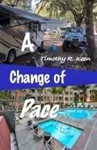
The cover sets the stage for this light romantic comedy about a fish out of water. Besides jumping from action/adventure to romantic comedy, I also did the cover artwork myself. I had used the same studio for the previous four books but this one seemed too simple for their expertise (they specialized in hand-painted fantasy art). Thus, the cover features the motorhome I was living in at the time and my old Land Cruiser, but I never lived in an upscale apartment in my life. That part is fantasy.
I love writing novels because it’s like binge watching several seasons of a favorite show and getting to know the characters intimately. There is so much that can’t be squeezed into the final text. Still, it can be fun to explore a stranger’s life for a few days, a span of time too brief to really get to know them, yet long enough to reveal something significant about their lives.
I took a break from writing novels to write a series of short stories that shared a common theme, which developed while working on them. I collected them together into Class of 1974. Imagine the different lives of people who graduated high school the same year, but had nothing else in common; until they all won the lottery.

These stories share two common themes: the title implies that the stories are tied to a rather dismal year in recent American history; the second commonality is more dependent on luck. I created the cover from a stylized Escher staircase showing people going nowhere, which seems appropriate for my cohort.
I think every writer should write short stories between major works. It’s like writing practice. And short stories are a great break from the concentration necessary to complete a novel, not to mention the lengthy timeline. I think the idea for Mirror Images originated in a dream (I can’t remember for sure) with a lot of images flashing past, nothing recognizable; it may have been my waking memory of a series of static dreams. At any rate the eventual result was a collection of stories sharing as many mirror metaphors as I could think of.

I fell in love with this photo I found on Shutterstock because it conveys so much in a simple black and white format, and it was a large image so it could be used for the entire paperback cover. Mirror Images contains a couple of stories I don’t care for (unhappy endings) and several I loved writing and enjoy reading over and over. I’d love to hear what you think.
That’s enough for this reboot post. Next time we dive deep into science fiction.
Publications Reboot
INTRODUCTION TO PUBLICATIONS
I’ve made a slight adjustment to my web page. Publications will now be automatically updated like a blog post (aspirational at best). This change will allow me to add comments upon reflection of my writing, which is an evolving process; however, it also gives me an opportunity to standardize the web page–I hate inconsistencies of every kind.
This first post in the Publications category is a summary of what was on the old web page. I’ve added a little here and there. Let’s begin at the beginning…
THE UNVEILED SERIES

Awakening of the Gods is the first book I wrote. I was inspired by watching documentary shows about ancient aliens. It was supposed to be a short story, but then well… I felt like the story ended without full closure even though it was meant as a single novel.
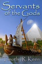
I became interested in the history of the fictional Inauditis people while writing Awakening, so I explored their ancient background in Servants of the Gods. This was fun to write because of our poor knowledge of what society was like 47000 years ago. I also had the opportunity to work with a professional illustrator, who produced the great cover from my description.

I wrote a clever ending for this story, which required that I write a third book in the series. In truth, these books were very enjoyable to write. Exiles of the Gods picked up the story shortly after Awakening with the same characters, but the central character became Pedro who happened to be the Pope.

The most enjoyable aspect of writing Exiles was integrating time travel into the developing story. It was very complicated and may be difficult to follow during a casual read. Of course, having introduced or at least implied the existence of malevolent actors on the world stage, I put a hook in at the end that required writing a fourth book to close the story.
The story became even more complex with the introduction of more players in War with the Gods.

It was worth the effort because the entire story was wrapped up, and I even managed to introduce God, or the nearest thing to it. The fascinating aspect of writing these books was how it forced me to think seriously about my beliefs. It has been suggested by a friend that this series is the basis of a religion. I hope not.

Recent Comments